Depending on the element you are working on from the Science program viewer, the Detailed element editor widow will change into the relevant display.
Observation Component Editor
The observation component editor is accessed by selecting the observation component in your science program, and is shown below.
The relative priority of this observation, compared with other observations in the same science program, is set using the High/Medium/Low buttons. See more details on how the priority affects execution and to add observations into groups. If not already defined, you can edit the observation name to make the science program viewer more understandable (normally this will be the science target name).
The Save button accepts the latest changes and stores the program to the local database, and the Close button closes the science program editor (saving any changes to the local database).
Phase 2 Status indicates the state of the observation through preparation. The status can have the following values:
- Phase 2 - The observation is in Phase 2 preparation. This is the default when the observation is created.
- For Review - The PI has finished the Phase 2 preparation and the observation is ready for review by NGO staff. The result of review is "For activation" or back to "Phase 2" for more work.
- For Activation - The observation has been successfully reviewed by NGO staff and it is ready for final review by Gemini staff. The result is "Prepared" or "On hold", or back to "For review" for further changes.
- On hold - The observation has been 'verified' but is not to be queued, e.g. it is waiting to be used as a ToO trigger.
- Prepared - The observation has passed its final review and is now considered fully prepared to be executed at the telescope.
- Inactive - The observation is not needed, has never been executed, and should not be queued.
Exec Status indicates the state of the observation through execution. The status can have the following values:
- Ready - The observation ready to be scheduled/executed.
- Ongoing - Execution is in progress.
- Observed - The observation has been executed.
The combination of Phase-2 status and Execution status determine the color of the observation icon.
QA state is set by Gemini staff after Quality Assessment of any data taken (see more details of the QA process). The values are:
- Undefined - no data taken or data not yet assessed.
- Pass - The quality assessment has been performed on the data. It meets the science needs and has therefore passed QA. The time used is charged to the program.
- Usable - quality assessment has been performed on the data. It does not meet the PI's science needs but might be usable by someone else (via the archive). The time is not charged to the program.
- Fail - The quality assessment has been performed on the data. It has failed QA and will not be archived. The time is not charged.
Observing Time gives all of the time charges for the observation. Different times are charged to the program or to the partner based on the observation class and the Quality Assessment.
Time Correction Log is used by Gemini staff to make adjustments to the automatic time accounting based on the QA of the individual datasets.
Target Component Editor
The detailed component editor containing the target list for an observation is accessed in the usual manner, by selecting the target component in your science program, and is shown below:
In normal circumstances, the target name and coordinates will have been extracted from the Phase I proposal, and will be shown in the top panel. The coordinates can be refined by editing the RA/Dec boxes in the Target Environment panel or by dragging the base position in the Position Editor graphical display.
The target name should contain alphanumeric symbols and blank spaces only, as some other symbols (e.g., brackets) can be interpreted as commands by the observing system.
If the observation is of a new target, the observation element is created with an empty telescope targets component and the science program viewer displays a placeholder (RA: 00:00:00.00 (HH:MM:SS.s) Dec:00:00:00.0 (DD:MM:SS.s) (J2000)) until an object name is given. When online, target coordinates and motion parameters can be obtained by querying the Simbad database by either pressing Return in the Target field, or by clicking on the magnifying glass.
![]() Note: the only supported coordinate system is J2000!
Note: the only supported coordinate system is J2000!
The scheduling time is used to determine the coordinates of nonsidereal targets, and defaults to the middle of the semester. This field is inactive for sidereal targets.
Target brightness information is entered in the middle panel, and is used as input to the ITC and to determine guide star viability. This information can be deleted by clicking the red X to the left of the string. Target brightnesses are entered as value:bandpass:system triples (see figure above). To manually enter a new brightness, select the bandpass from the pulldown menu to the right of the box labelled "Select" and then enter a value into the box. Additional entries to the table can be added by clicking on the green + below the list. An entry can be deleted by clicking on the appropriate red X. The Brightness table is automatically sorted by wavelength.
Target motion parameters are listed in the box below the coordinates. Proper motions are specified as µαcosδ and µδ, expressed in mas/yr (10–3arcsec/year) along with the epoch of the proper motion. The parallax should be given in mas. The apparent line-of-sight velocity may be specified as either radial velocity (RV in km/s) or redshift (z). Some or all of these parameters may be filled in automatically with Simbad and guide star queries.
The upper panel displays the target list. Each position has a tag associating it with the base (telescope) or one of the wavefront sensors (WFSs). The specific WFS tags are associated with telescope offset positions using the offset iterator. The User tag is not associated with a WFS and is normally used to give the coordinates of stars to be used for peak-up before blind-offsetting to a faint target. If you wish to change the tag type for a particular position, select the item in the target list and choose the new tag type from the pull-down list at the bottom of the top panel. The distance between the base position and the other targets is listed in arcminutes, and all of the known magnitudes are listed for each target (note you may need to use the horizontal scroll-bar to see all the values).
You can add or remove items in the target list (except the base position) using the add/remove/duplicate buttons. Pausing the cursor over one of the buttons will reveal adescription of the button's function. A summary of the buttons is given below.
 |
Add new empty target or magnitude |
 |
Remove selected target or magnitude |
 |
Copy selected target to buffer |
 |
Paste target buffer into selected target |
| Duplicate selected target | |
 |
Activate/deactivate selected guide star |
Targets can be copy/pasted between target components in different observations, including observations in different programs.
The Duplicate button will copy the information of the selected target and copy it to a new line in the table. If the base position is duplicated, then the new target has a User tag. If another type of target is duplicated then the new target has the same kind of tag as the original but the running number is incremented. For example, if target PWFS2 (1) is duplicated then the new target has the tag PWFS2 (2).
Duplication is especially useful for preparing AO observations in which the AO correction is calculated from the science target. In these cases, the target and guide star must have the same name and coordinates.Therefore, one can simply duplicate the target and then set the tag for the appropriate type of wavefront sensor. If using Altair, then the guide star tag should be AOWFS whilst, if using NICI then the guide star tag is OIWFS.
The Auto Guide Search menu is used to change the WFS used by the automatic guide star algorithm. By default it suggests the most likely guide star needed for the instrument and AO system (if any) in the observation.
The Manual GS button will open the position editor (if it is not already open) and then open the Catalog Query Tool for doing manual guide star searches from either the UCAC4 or PPMXL catalogs.
Non-Sidereal Targets
For details on observing non-sidereal objects please see the Non-Sidereal Targets page.
Guide Star Quality
The guide star "Quality" provides an estimate of whether the brightness of the guide star could impact the delivered image quality:
 |
Guide star is bright enough to deliver the requested image quality in the specified conditions |
 |
Slower guiding required; may not deliver the requested image quality in the specified conditions |
 |
Slower guiding required; will not deliver the requested image quality in the specified conditions |
 |
Guide star is very faint; we may not be able to guide in the specified conditions |
 |
Guide star is too faint (or too bright) to guide in the specified conditions |
The guide star quality details are displayed at the bottom of the Target Environment when the guide star is selected. The limiting magnitudes for the selected wavefront sensor are shown at the right, and hover-over text gives estimates for the different guide speeds (fast, medium, and slow).
The guide star quality is meant to be a guideline only, providing a warning when guide stars may be of inadequate brightness for the requested image quality and observing conditions. In practice, the guide speed and impact on delivered image quality will depend on the accuracy of the guide star catalog magnitude and the specific conditions during the observation.
Source Parameters
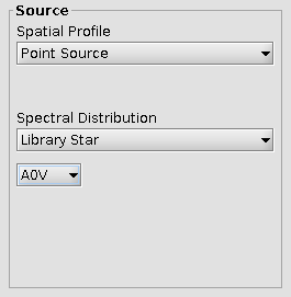
Since 2015B, the OT includes an interface to the Integration Time Calculators (ITCs), which requires specifying the source morphology and spectral energy distribution. These may be set in the Source panel to the right of the Magnitudes panel. Note that you may need to expand the OT window horizontally to see the Source panel:
 |
 |
 |
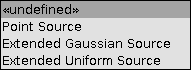
The source Spatial Profile may be one of:
- Point Source, where the integrated brightness is specified by the magnitude table
- Extended Gaussian source, which will reveal a field to specify the FWHM in arcseconds, and the magnitude table describes the integrated brightness
- Extended Uniform Source, where the magnitude table describes the surface brightness in magnitudes per square arcsecond
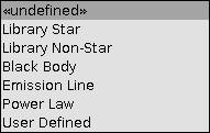
The source Spectral Distribution may be one of:
- Library Star, which reveals a drop-down list of stellar templates
- Library Non-Star, which reveals a drop-down list of SED templates, including: Elliptical Galaxy, Spiral Galaxy, QSO, HII Region, Planetary Nebula, etc.
- Black Body, which will reveal a field to enter the source temperature in Kelvin
- Emission Line, which will reveal 4 fields: Line Wavelength (microns), Line Width (km/s), Line flux (W/m2), and Continuum flux (W/m2/um)
- Power Law, which will reveal a field to enter the power-law index
- User Defined, which will reveal a list of all SED files attached to the OT
Integration Time Calculator
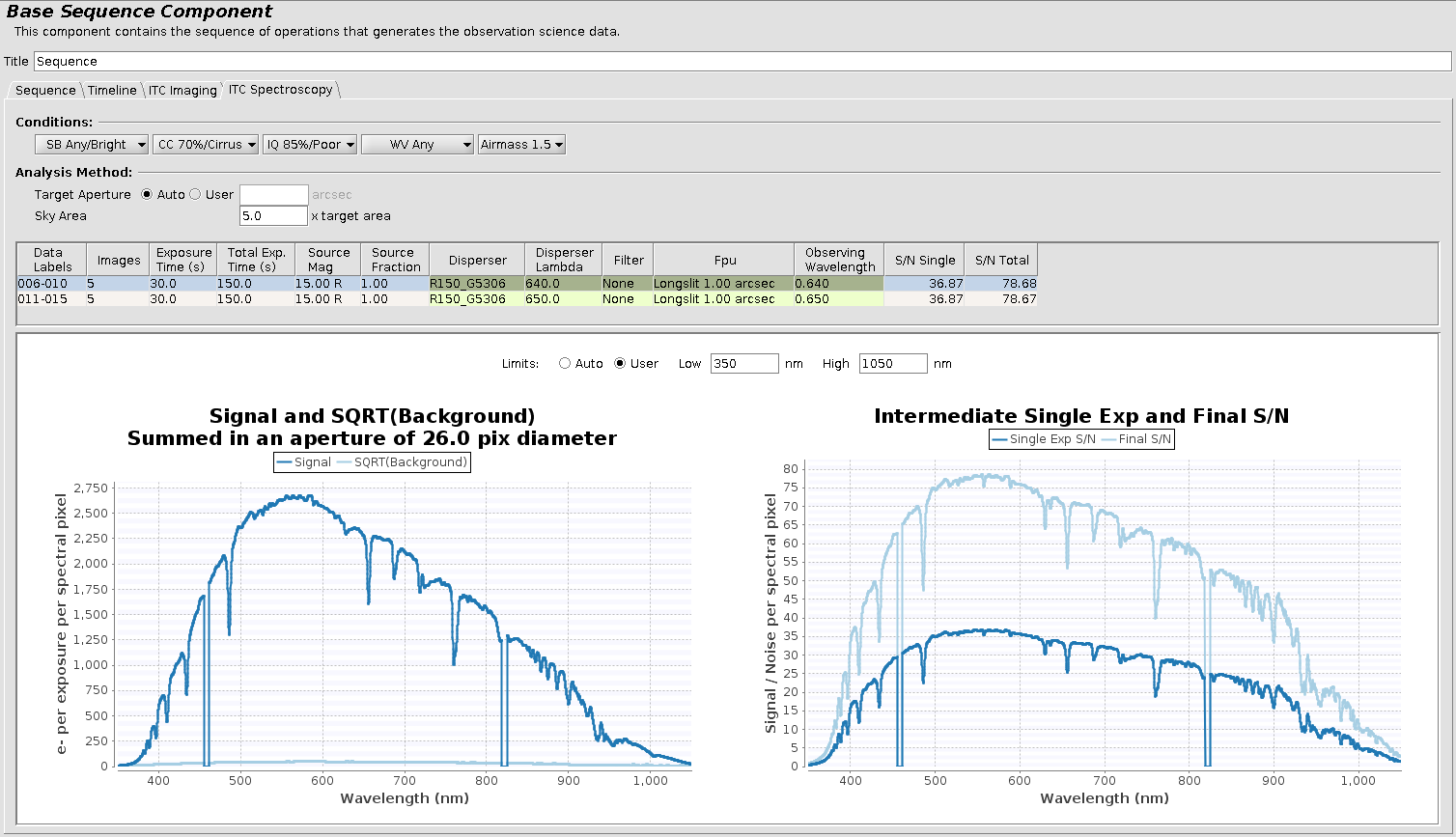
The OT includes an interface to the on-line Integration Time Calculators (ITCs). The ITC tabs are found in the Base Sequence Component, to the right of the Timeline tab (see figure below). Instruments which only support imaging (i.e. GSAOI) will only show an Imaging tab, and instruments that only support spectroscopy will only have a Spectroscopy tab. Instruments which can do both will have both tabs, although depending on the observation, only one may be populated.
Source
The ITC uses the spatial profile and spectral energy distribution defined in the Target Source Parameters section. If either is undefined the ITC will return an error.
When using an Extended Uniform Source spatial profile, the source magnitude will be interpreted as magnitudes per square arcsecond.
Conditions
The top-left of the ITC tabs include drop-down menus to select the observing conditions to be used for the ITC calculations. These default to the values specified in the "Observing Conditions" component, but may be modified to see how the predicted results will change under better or worse conditions. Values different than the approved conditions are indicated in red.
Analysis Method
The top-right of the ITC tabs allows specifying the target and sky aperture sizes. The target aperture defaults to "Auto" which should yield the best S/N. See the ITC Documentation for additional information.
Configuration Table
The bottom of the ITC Imaging tab, and the middle of the ITC Spectroscopy tab shows a table of input and output values, with one line for each unique instrument configuration in the observation. If a target has multiple magnitude bands specified (in the Target Environment), the ITC will chose the Source Mag as the one closest in wavelength to the science wavelength. The Source Fraction is calculated based on the size of the offsets; offsets larger than half the field of view are counted as off-source. The Peak counts estimate the peak pixel value (in electrons), used for predicting saturation. The S/N is listed for a Single exposure, as well as the Total for when all the data from a single configuration are combined.
Graphs
The bottom of the ITC Spectroscopy tab will also show graphs of signal and background, and signal/noise ratio as a function of wavelength. The graph ranges may be configured by setting the User Limits at the top of the graphs, or by drawing a box on the graph, moving from left to right, to zoom in on a portion of the graph. Drag from right to left to return to the default zoom level.
Offset Iterator
The offset iterator provides a convenient means to specify telescope sequences e.g.mosaics, dithers, nods. The main features of the offset iterator are identified in the figure below:
The coordinate system for offsets is defined as (p,q) where q is always parallel to the detector columns (or spectrograph slit) and p to detector rows (or orthogonal to the slit). The sketch in the lower left corner of the offset iterator is a useful reminder. Offsets are always entered in arcsec relative to the base position. For example, using a long-slit spectrograph like GMOS or GNIRS, an offset of (0,q) where q is any real number is always along the slit regardless of the position angle on the sky.
This (p,q) coordinate frame, and the offset positions, rotates with the image rotator. Thus only one mosaic is required regardless of the specified position angle. Similarly, if the base position is moved (i.e. translated) the offsets will move with it. With an offset pattern displayed in the position editor, you can drag the instrument rotation angle or base position to see this behavior.
The concept behind the telescope offset iterator is similar to the instrument iterators. You build up a sequence of telescope offset positions in an iteration table.The table columns are (a) Index, (b) p offsets, (c) q offsets and (d) the guide state (on/off). Table rows correspond to iterator steps. At run time, all the values in a row are set at once.
As many offset positions as desired may be entered, and the ordering of the list (the execution order) can subsequently be modified using the up and down arrow buttons. The selected offset, highlighted in green, can be moved up or down one step using the yellow arrows, or moved to the top or bottom of the list using the arrows with a bar. You can select and display (or re-order) multiple steps at once. To select several adjacent steps, click on the first one in the iteration table then shift+click on the last one; all steps in between will be selected (highlighted). To select non-contiguous steps ("disjoint sections"), select the first step and then ctrl+click on any others that you wish to select.
Steps in the list can be removed individually with the single red X button, en masse with the red XX button, or new steps may be added with the green + button. The values of a particular (highlighted) offset can be changed using the p and q editing boxes.Often it will be more convenient to change offset coordinates interactively in the position editor by dragging any offset as the science fields of view corresponding to the offsets and WFS probe vignetting are also displayed.
The "Grid..." button in the lower right of the offset iterator allows rapid creation of rectangular grid patterns. Set the offset of the initial position, the spacing and grid dimensions, then select create. Subsequent grids (e.g. to map an area of nearby sky) can be appended to the offset list. The order of steps in the list can be modified as described above to create arbitrarily complex patterns.
The "Random..." button can be used to quickly create sequences of random offsets that populate a square of the specified maximum offset in p,q.
If there are steps in the offset table where the guiding is listed as "off" this means that the WFS will not be moved from its previous position (i.e. it will not compensate for the telescope offset and will not attempt to stay locked on the star). This is useful if you wish to maintain the same illumination (vignetting) pattern on the detector e.g. for sky frames.
From the offset iterator it is possible to step through the sequence and display the science area and WFS probe positions in a (rudimentary) "playback" mode:
- Configure the Position Editor to display the science FOV only at the selected position:
View > Science Display > Display Science FOV at > Selected Position. - Configure the Position Editor to display Base, Offset, Science and the WFS FOV.
- Select (highlight) the first step in the offset list.
- Step through the offsets using the down-arrow key on your keyboard.
- The position editor viewer will update at each step.
The "Advanced Guiding Options" tab is used to define the guide state of each guider individually, and should not be necessary in normal use.
The Save button accepts the latest changes and stores the program to the local database, and the Close button closes the science program editor (saving any changes to the local database).
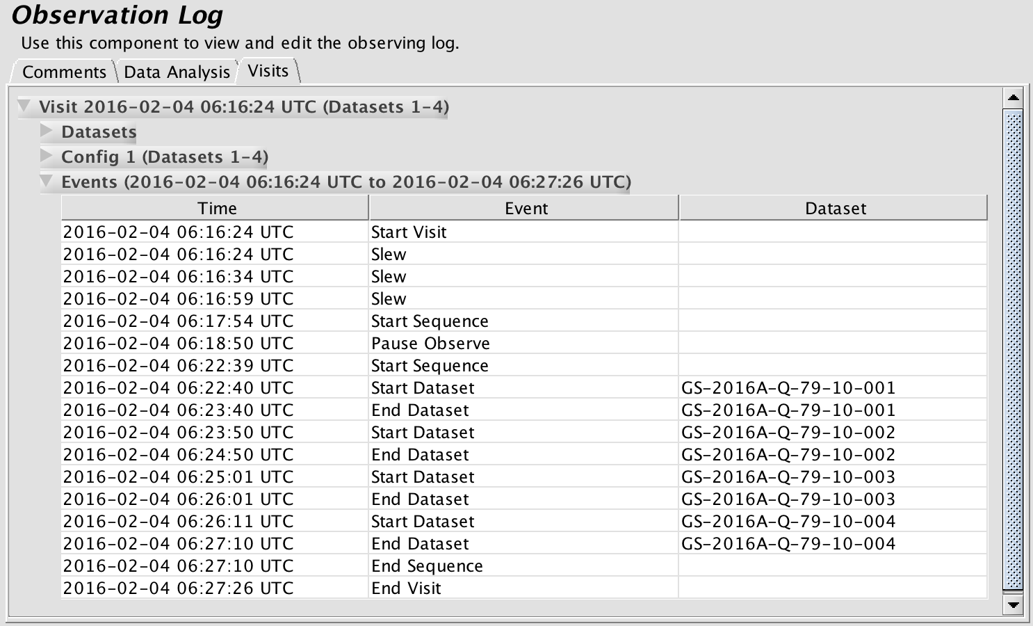
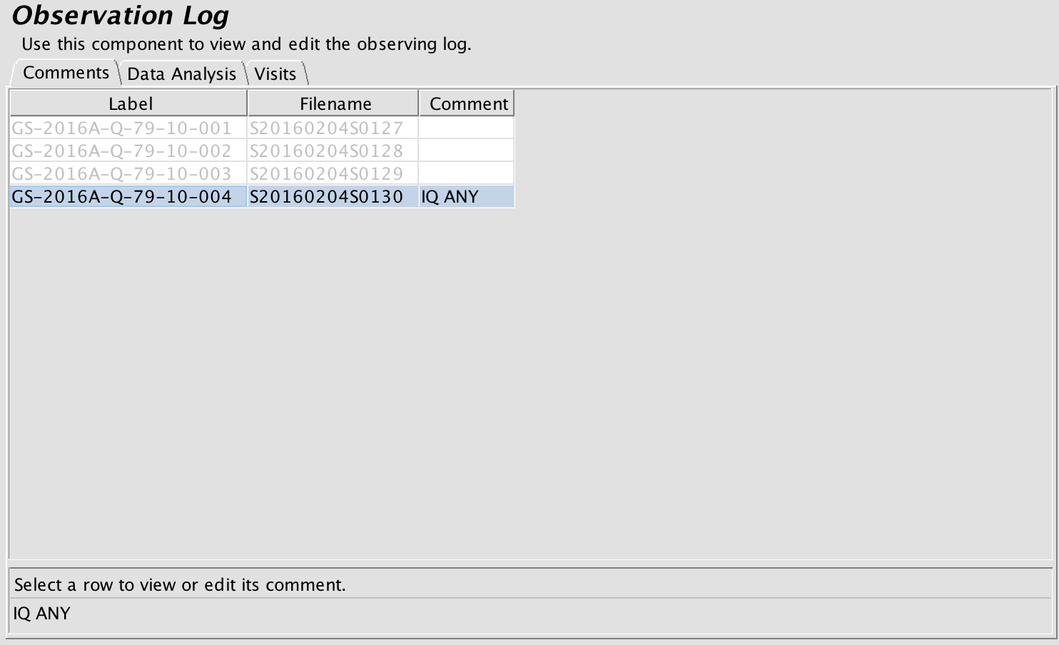
Observing Log
The Observing Log node provides details about the execution of the observation.
The Comments tab gives the data labels and FITS file names for the executed steps and comments entered by the observer. Click on a line to see the full comments in the box at the bottom of the tab.
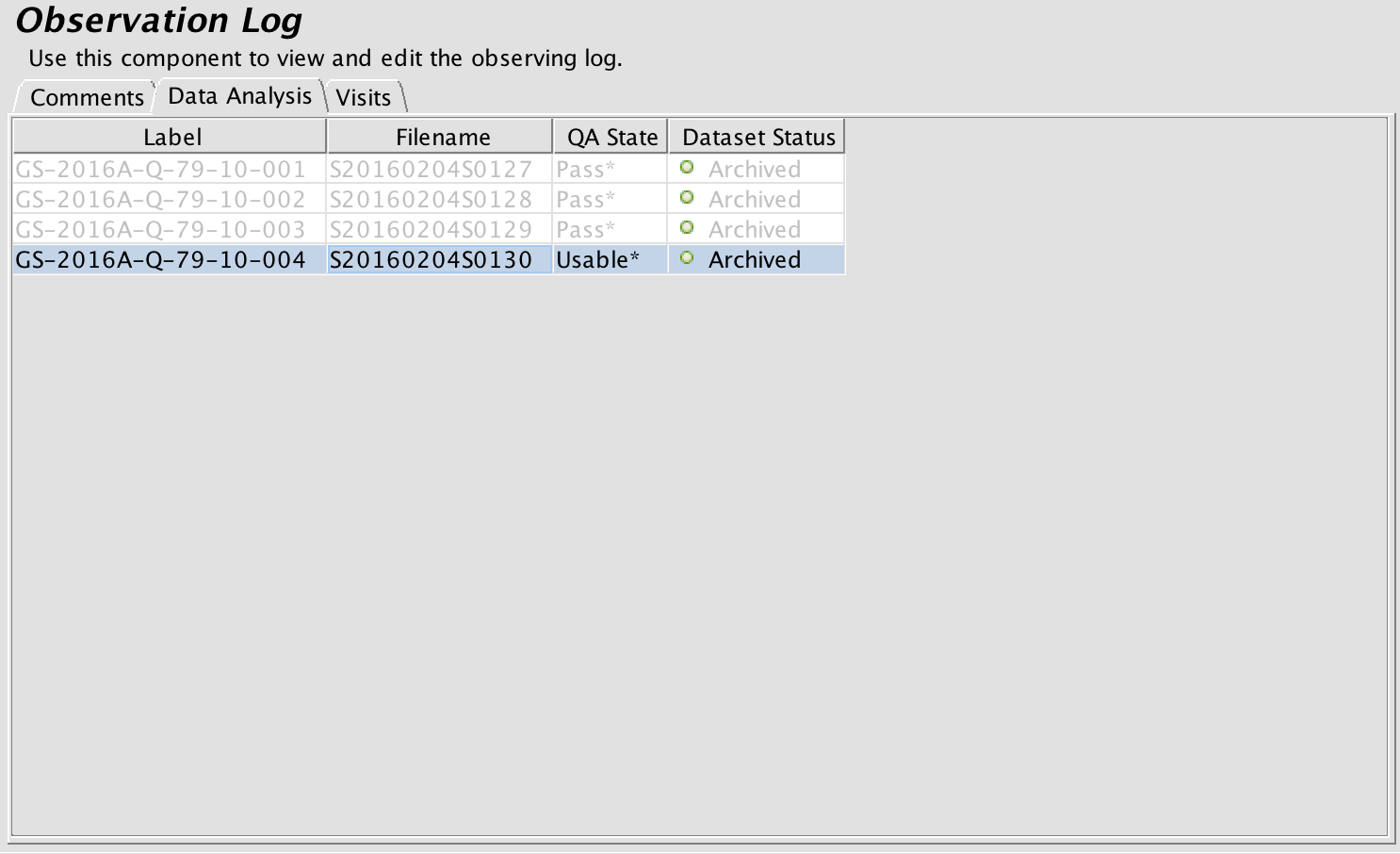
The Data Analysis tab is used to set the quality assessment state, which also updates the FITS headers if the files are still in Gemini's short-term storage area. The tab also gives the status of the FITS file in the Gemini Observatory Archive.
The Visits tab gives details about the events that occurred during the observation visits. Configuration details and timestamps for each event are given. This information along with the quality assessment flags ared used by the OT to calculate the time used.