GMOS solutions documentation 

Germán Gimeno & Verónica Firpo, Gemini Observatory   
Aug. 2018, La Serena. Last update July 2022

This tutorial will provide some advanced tips on GMOS-S data reduction based on IRAF that will hopefully help to solve some of the most serious issues that may arise as a consequence of the problems related to the detectors and the instrument. These solutions were compiled from the numerous requests from the users within the last few years. These are not definitive, fail-proof solutions; they may work well with some datasets and not so well on others, depending on what was the initial observing strategy, the quality of the raw data, etc.

Familiarity of the user with the gemini.gmos iraf package is assumed.

Table of Contents

• Dates & Status of the detectors

  • Dates
  • Status of the detectors

• How to solve problems with images.

  • Science imaging or MOS preimaging (full frame)
    • Case 1: point source(s) or sparse field
    • Case 2: extended objects, and/or non-dithered images
    • Case 3: imaging treatment to mimic the faulty amplifier#5

• How to solve problems with longslit spectroscopy.

  • Science longslit spectroscopy
    • Case 1: The correct way to use QE correction

• How to solve problems with MOS spectroscopy.

  • Science MOS spectroscopy

• How to solve problems with 3D spectroscopy.

  • Science IFU spectroscopy

Appendix

• A.1 Bad columns treatment (all modes) on “Hamamatsu/EEV” detectors
• A.2 Amp5 bad column saturation banding problem
• A.3 Biases structures

Dates

• March, 2022

  Although the CCD1 CTE issue was fixed, the noise problem on CCD2 and CCD1 persists. An intervention is being planned, in order to to permanently solve the issue. In the meantime, the observations were resumed in a "limited" mode.  To minimizing the effects of the bad amplifier#5 on science data and/or to place targets or spectral features of interest on other parts of the detector, an appropriate dither strategy was planned.  As much as for imaging and longslit or for MOS and IFU-R, the same strategy was been applied as well.  The main additional difficulty is the wavelength calibration since some arc lines are wiped out and the autoidentify task may fail. In this case, the lines identification has to be done interactively. For IFU-2, it is more complicated since amp5 is a relatively larger portion of the spectral interval and calibration would in general fail or be quite poor. Nevertheless,  this is been looking into it.

• February, 2022

  After the uncontrolled warmup caused by the general power failure at CPO on January 28th, the GMOS CCDs have been in a bad state with abnormally high counts on amplifier#5, plus high noise structures on the rest of CCD2, and the re-appearance of the CTE problem on CCD1.

• April, 2021

  After the short GS telescope shutdown at the end of March, new GMOS-S Nod and Shuffle test data showed that the CCD1 CTE problem spontaneously gone, and the CTE is again within specification in all three chips. All Nod & Shuffle observations are resumed.

• January, 2020

  After the short thermal cycle on Dec 18, 2019 to replace the coldhead's displacer, the charge smearing in GMOS-S CCD1 re-appeared as shown in the screenshot of the N&S dark from April 2019. The N&S mode and IFU-2 and IFU-R observations were affected. 

• June, 2019

  After a successful intervention in the CPO Instrument Lab where the ESD board was replacement, the charge smearing despaired. GMOS-S was back on the telescope and fully operational in all science modes, including Nod & Shuffle. 

• May, 2019

  Unfortunately, after performed a new thermal cycle on GMOS-S in order to get the transitory CTE problem fixed it did not work as expected and GMOS CTE showed no improvement: CCD1 still showed strong charge smearing in N&S data, and CCDs 2 and 3 some mild smearing. 

• April, 2019

  The charge smearing has reappeared in GMOS-S CCD1 (screenshot of Nod&Shuffle Dark is attached). 

• June, 2018

  After a performed a controlled thermal cycle GMOS-S detector came back fine and the bias images taken after the cooldown showed that the bright structures were completely gone and readout noise is back to its nominal value (~4e-). The CTE was fine in the three chips and charge smearing that had reappeared in May was no longer present in CCD1. 

• April, 2018​

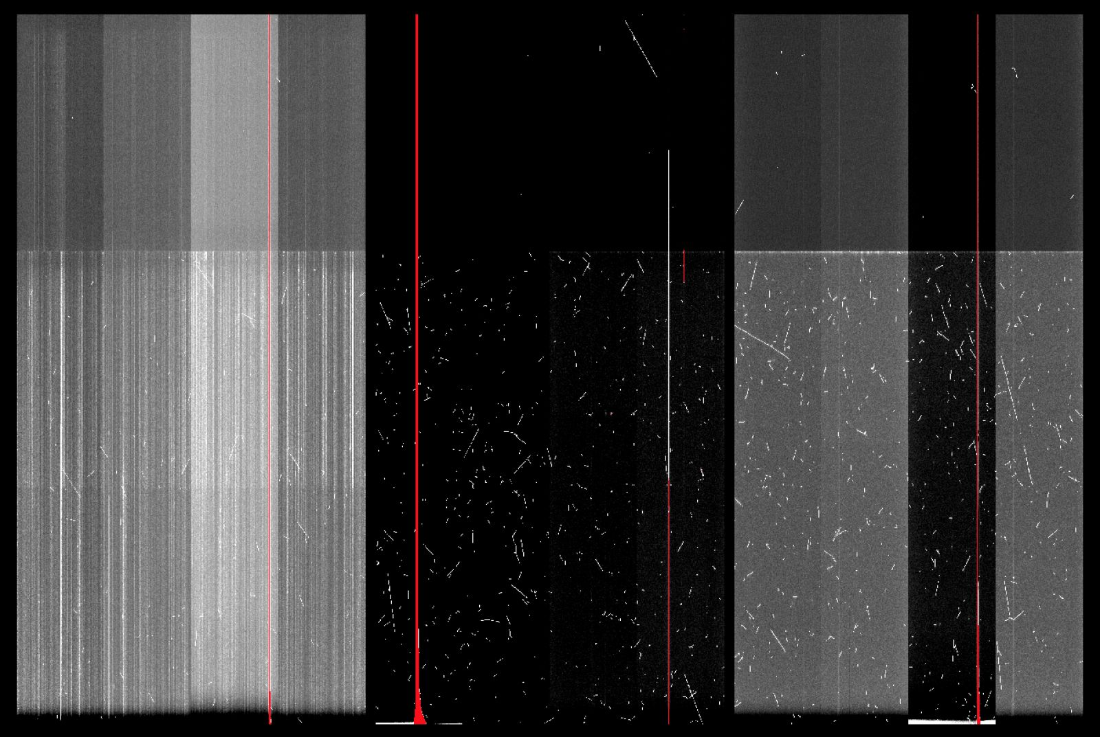
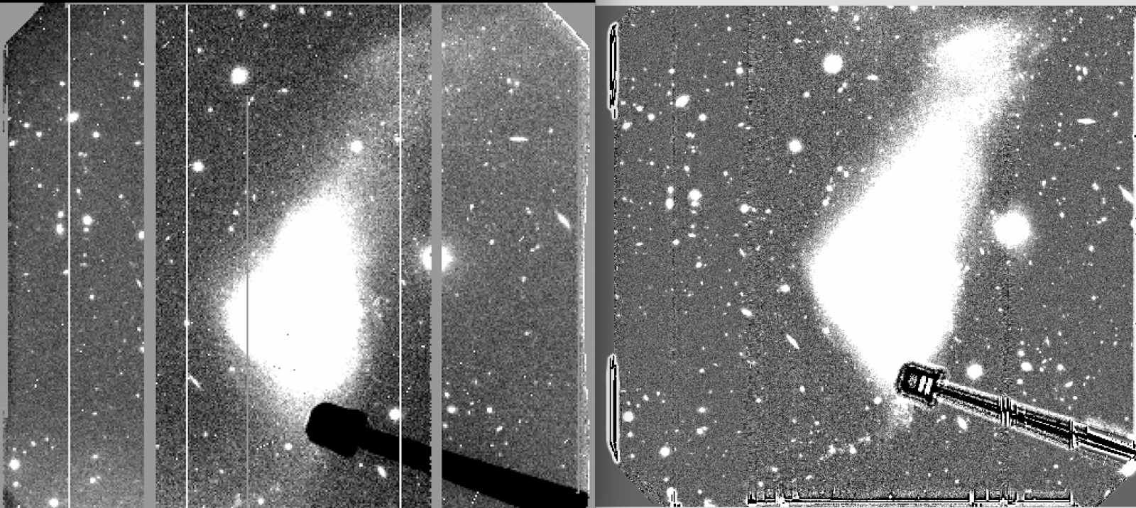
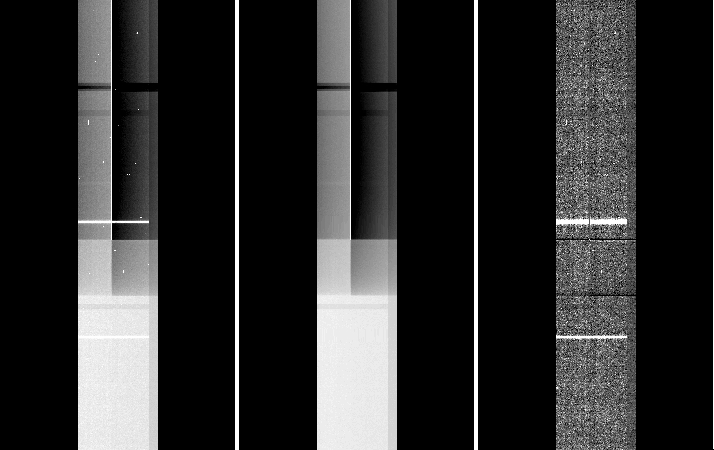
  On April 3, the CCD1 started showing charge smearing at a very low level (1-2 counts level). It became more evident in long exposures caused by numerous cosmic ray hits (3-5 counts level). On April 28, after a full thermal cycle of the dewer, the charge smearing problem disappeared but the bias pattern which existed from September 30, 2016 to February 21, 2017  reappeared in CCD2 although they were not as strong as the previous ones in 2016. PIs with data taken after April 28, 2018 should use biases taken after that date. It recommend to use the bias frames taken on the same day to properly remove the pattern shown in the figures.

 Left: GMOS-S r-band raw image taken on 4/29/18, middle: Bias pattern in CCD2, right: reduced image after applying bias subtraction

• February, 2017 

  The GMOS-S bias structure reported previously in November 2016 were spontaneously gone, after a thermal cycle.  Biases are mostly clean only some residual vertical fringes about one or two counts over the bias level. The known bad columns persist (amps #3, #5, #8 and #11). Noise values are the normal ones (~4e- rms).

• November, 2016 

  GMOS-S detector developed a new structure on bias frames, especially on CCD2, this being harmful in the following cases:
• Imaging of very faint targets;
• Imaging of low surface brightness structures;
• Spectroscopy of faint targets; 
• Also the number of bad columns has increased with each thermal cycle. The advise to use bias frames taken after September 30th for data taken since that same date, preferably as close as possible in time.

• September, 2016:

  A sporadic appearance of a hint of CTE issues on CCD1 was noticed in N&S observation from. A slight charge smear is evident in comparison with CCD2 and CCD3, in a 8-cycle N&S exposure. In contrast recent 17A 20-cycles N&S exposures show no signs for a degraded CTE.

• September, 2016:

  More new features appeared on GMOS-S raw data, the most notable features being vertical fringes on CCD2 and CCD3. The dominant bias features are not uniform but highly structured (bright, vertical lanes). The noise is enhanced at the location of these features, which can affect spectroscopy of faint targets, particularly in MOS and IFU observations.

• End of June, 2016:

  New bad columns developed and some bar-like vertical structures appeared having a few counts above the mean bias level on CCD2.

• May, 2015 - July, 2015:

  Another problem namely a charge transfer issue affecting CCD1 in Nod and Shuffle data. The end of July 2015 the CCD1 CTE problem was spontaneously gone and permanently fixed the saturation "banding" problem.

• February, 2015:

  A banding issue and accumulating spurious charge on amplifier #5 (in CCD2) and bad columns appear.

• June 11, 2014:

  The saturation banding in binned data effect is a lowering in counts (with respect to the bias level) that happens when one or more pixels saturate, affecting the whole amplifier width. 

• August 22, 2014:

  GMOS-S was back on sky after the controller backplane was replaced during the telescope shutdown, and the problem was gone.

Status of the detectors

=> Status and Availability

• CCD1: CTE issue fixed. One bad column, saturating, 5 pix wide, on amp#3.
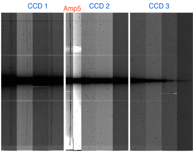
• CCD2: high noise structures are present. Amp#5 is completely unusable (see the document http://www.gemini.edu/sciops/instruments/gmos/GMOS-S_badamp5_ops_2.pdf). Two bad columns on amp#8 (first one 3pix wide, ~300 counts; second one 5 pix wide and saturating in ~25 minutes).
• CCD3: high noise structures are present. One bad column on amp#11 (saturating in ~20 minutes, 5 pix wide).

Science imaging or MOS preimaging (full frame)

Case 1: point source(s) or sparse field

1.A) One simple procedure is to reduce the images the standard way:

1. Subtract overscan [1] and bias [2].
2. Mask the bad columns [3].
3. Perform the QE correction on the twilights and the science frames (task gqecorr)
4. Perform the flatfield correction of science frames (and fringing [4] correction if suitable) using the QE corrected twilights
5. Mosaic the images (task gmosaic).

Ideally at this point the processing should be complete; however it is observed that many times residual gradients remain. In order to correct for this, there are several possible approaches.

       6.  Build an illumination correction frame from the resulting final science image (from step 5. above). First masking and removing all sources on the image (e.g. tasks objmasks and fixpix, or manually). Then smoothing (using sigma values ~30 have proven to work fairly well) and normalizing the result to get the illumination correction frame. Finally divide the science image by this illumination correction [5].

       7. Co-add the images (task gemcombine).

1.B) Another way is to build the flatfield from the background sky of the actual science frames by means of the median image. This assumes a sequence of dithered images, where the dither amount is greater than the size of the source(s) of interest

1. Subtract overscan [1] and bias [2].
2. Mask the bad columns [3].
3. Perform the QE correction on the twilights and the science frames (task gqecorr)
4. Perform the flatfield correction of science frames (and fringing [4] correction if suitable) using the QE corrected twilights.
5. Build a median image from all the flatfielded science images [6] and normalize it to obtain the illumination correction frame. This should not have any residual source on it. The IRAF task gemcombine can compute the median for GMOS MEF images.
6. Perform the illumination correction with this normalized median frame [7].

1.C) However, we found that a minimum-combined image gives better results than the median for the flat field since the removal of residuals from the sources is better. For this to work correctly, the steps are:

1. Subtract overscan [1] and bias [2].
2. Mask the bad columns [3].
3. Perform the QE correction on the twilights and the science frames (task gqecorr)
4. Scale all images to the same value of the background sky level. This is very important for the procedure to work effectively. In IRAF use the task imstat over a selected background region, common to all images in order to find the mean value over that region. Then multiply by the scaling factor (if all images have the same exposure time this will be close to 1)
5. Use the IRAF task gemexpr to compute the minimum-combined image: for a three image set for example:

gemexpr "min(a,b,c)" result.fits scaled_image001.fits scaled_image002.fits scaled_image003.fits

where a,b,c stand for the input images (scaled_imageXXX)

        6. The result image needs to be normalized before using it as flatfield:

giflat result.fits flat_result.fits

where flat_result is our final flat, that can now be used as any regular flat field image. After this, display the resulting flat and inspect visually whether there are any residuals.

In case there are residuals, they can be removed manually with the task imedit

imedit flat_result[SCI,n] aperture=circular radius=100

where n is the extension number. This allows to interactively modify pixel values in the image; in thee example above, it will replace the residuals with a 100-pixel radius circular background over the cursor position upon a “b” keystroke (see the “help” of the task for more details).

      7. Perform the bad columns masking, mosaicing an coaddition as normal.

Example of a minimum-combined image (left) and a median-combined image (right). The former procedure provides better elimination of residuals (see 1.C)

Example of a flatfielded image using the standard procedure (left) and the improved flatfielding (right) described in the section "Case 1"

Case 2: extended objects, and/or non-dithered images

This is for images in which the dithering amount is smaller than the size of the target of interest (i.e. partially overlapping offset target positions on the FOV). Also for the case of non-dithered images (either point source or extended). The idea is to fit a 2D surface to the background and then use it as a flatfield image.

2.A) In many cases the procedure listed in 1.A) is also applicable for non-dithered images and some extended objects (provided their largest linear size is no more than ~30 arcminutes). This would be the first thing to try.

2.B) If you have extended targets, but with a sequence a dithered images in which the dither amount is larger than the largest source, the procedures described in 1.B) and 1.C) can work as well.

2.C) If 2.A) is not applicable or the result is not satisfactory, then

1. Subtract overscan and bias (same as above)
2. Mask the bad columns (same as above)
3. Fit a 2D surface to the background. If you have a sequence of dithered images, it is best to perform a median combined image (similarly as 3) above) and use this median image for fitting the 2D surface. It is also advisable to work with the individual extensions separately. For the fitting you need to use the available sky regions within the image.
4. Use the fitted, normalized 2D surface for flatfielding the science images.

Case 3: imaging treatment to mimic the faulty amplifier#5

Patch release of DRAGONS, v3.0.3, is available that offers an automated handling of GMOS-S amplifier #5 and also includes a few other bug fixes (https://www.gemini.edu/observing/phase-iii/reducing-data). 

The following tutorial shows a step-by-step imaging reduction but using IRAF which include a treatment for the bad amplifier#5 (see the document http://www.gemini.edu/sciops/instruments/gmos/GMOS-S_badamp5_ops_2.pdf).  The starting point is a raw images dataset consisting of:

- Science image(s) (for removing bad amp#5 satisfactorily, at least two images dithered in P= +/- 30 arcsec as described in the document linked above are necessary, three images recommended).

 - A set of bias images as close in time as possible. In particular, for science images affected by the noise patterns described in the document, biases with the same noise patterns are necessary for proper subtraction.

 - A set of twilight flatield images *from a single date*. This is very important. Do not mix single flatfield images from different dates.

This is the bare minimum, however it is strongly advised to use the bad pixel mask for correcting the bad columns. It is possible in any case to derive it from the science data. Alternatively, the bad columns can be masked manually as shown below.

If you already have a master bias and a master twilight (e.g. from a previous reduction), you can start off from step 3. 

Familiarity with IRAF and the ‘gemini’ and ‘gmos’ IRAF packages is assumed. Individual commands are depicted in IRAF command mode in console fonts, and can be copied/pasted into the IRAF prompt. More flexibility can be achieved by using them in program mode in cl scripts (gima.cl).

1. Process the biases:

gbias @bias_list.txt outbias="bias_out.fits"  fl_over+  fl_trim+  logfile="gbias.log" order=63.

order 63 is recommended for the overscan fit for GMOS-S.

IMPORTANT: whatever value you choose for this parameter, keep consistency throughout the reduction, i.e. use the same order for twilights and science. 

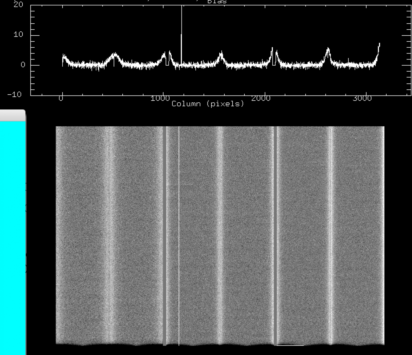
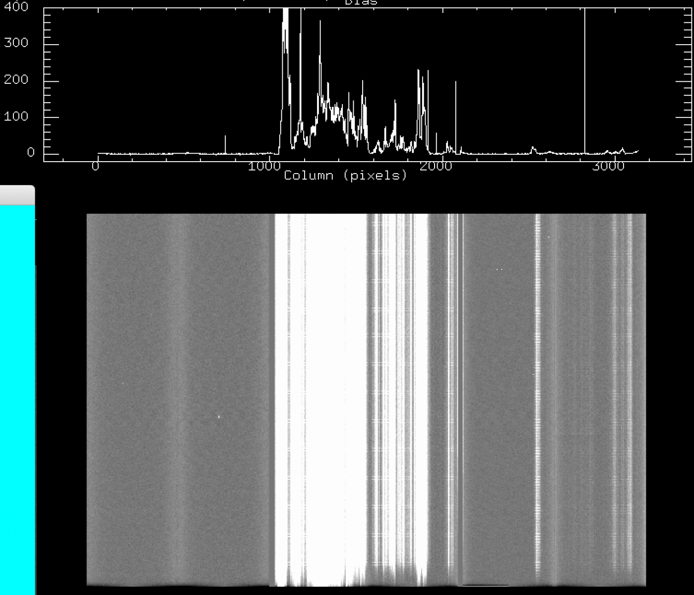
The result should be like the one shown in Fiigure 1. In this case, the bias shows the noise structures mentioned above and the faulty amplifier #5.

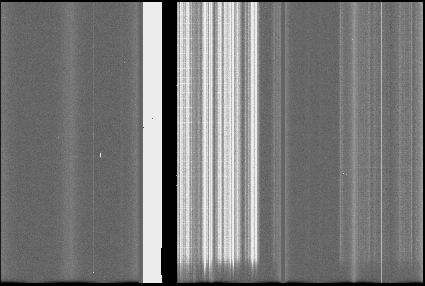
Figure 1: GMOS-S master bias frame

2. Process individual twilight flats (from the same observing date, as stressed above) into a master twilight flat (if you already have the master flat, skip to step 3).

This is done in three steps:

    a) Bias and overscan subtraction: 

gireduce @twilight_list.txt outpref="f" fl_bias+ fl_over+ fl_trim+ bias="bias_out.fits" order=63. fl_qecorr-

Note that we used the same order for the overscan fit as the bias, as indicated.

    b) Relative QE correction

This is the tricky step.  Fortunately there is now a script that does this automatically (not part of the IRAF package).

First build the list of the bias-subtracted raw twilights:

files fg//twilight_list.txt > qe_list.txt

Then run the script qemeasure_adv_YYYYMMMDD.cl:

cl < qemeasure_adv_YYYYMMMDD.cl 

(the YYYYMMMDD refers to the version date of the script). This will basically make a local copy of the file ‘gmosQEfactors.dat’ (which is located in IRAF directory ‘gmos$data’), compute the QE factors, insert them in this local copy of the factors file.

Then run gqecorr on the twilights, using this local file:

gqecorr @qe_list.txt qecorr_data=./gmosQEfactors_mod_tw.dat logfile='gqecorr_flat.log'

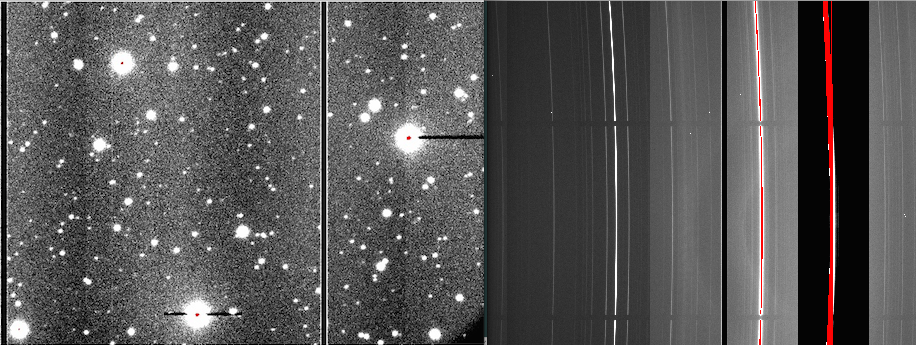
The output will be the individual QE corrected twilights (see Figure 2), with the “q” prefix.

Figure 2: r’ twilight before (left) and after (right) relative QE correction

  c) Combine the processed individual twilight flats into a master flat (giflat task):

giflat inflats='q//@qe_list.txt' outflat="Twilight.fits" fl_bias- fl_over- fl_trim- logfile="giflat.log”  fl_qecorr-

Note that the bias, overscan trim and qecorr options are deactivated since we already did that. This master twilight flat is normalized and corrected for relative QE differences between the CCDs.

3.  Process individual science frames: 

   a) Bias and overscan subtraction (gireduce task with fl_flat turned off)

gireduce @science_list.txt outpref='rg' bias='bias_out.fits' fl_over+ fl_flat- order=63. 

Note that we postponed the flatfileding for later. The files will have "rg" as prefix

    b) Relative QE correction (gqecorr task, with default parameters)        

gqecorr rg//@science_list.txt logfile='gqecorr_sci.log' 

4. Divide each of the processed science frames from step 3 by the master twilight obtained from step 2:    

gireduce qrg//@science_list.txt fl_bias- flat1=Twilight.fits logfile='gireduce_sci.log'

5. Mask extension [5]:

Eliminate unusable data from amp#5. The easiest way is to set every pixel value to 0:        

imreplace rqrg*.fits[5] 0.

Bonus: you can mask the bad columns on the rest of the extensions easily in this way, since their location is known (as of March 2022):

imreplace rqrg*.fits[3][226:235,*] 0.
imreplace rqrg*.fits[8][93:96,*] 0.
imreplace rqrg*.fits[8][134:143,*] 0.

 NOTE: this is for 2x2 binning  (typical for most imaging). If using 1x1 just multiply the above figures by two.

6. Frame:

This step is optional, but highly recommended for better quality of the final image. We multiply the images by the provided ‘frame2x2.fits’ file, which is zero outside the GMOS imaging FOV (you con just copy/paste the following block into the cl prompt).

NOTE: this file works with 2x2 binning only (a 1x1 version will be available soon).

ls rqrg*.fits > reduced.txt
string *list1
list1='reduced.txt'
while (fscan (list1, s1) != EOF){
                gemarith (s1,"*", "frame2x2.fits", "f"//s1)
                }

7. Mosaic the flat-fielded images:

In this scheme, deactivating both fixpix and clean will give best results:

gmosaic frqrg*.fits fl_fixpix- fl_clean-

Sometimes due to strong sky color variation, even after having performed the formal RQE correction, there could remain background intensity differences (see Fiigure 3) in the mosaiced images.

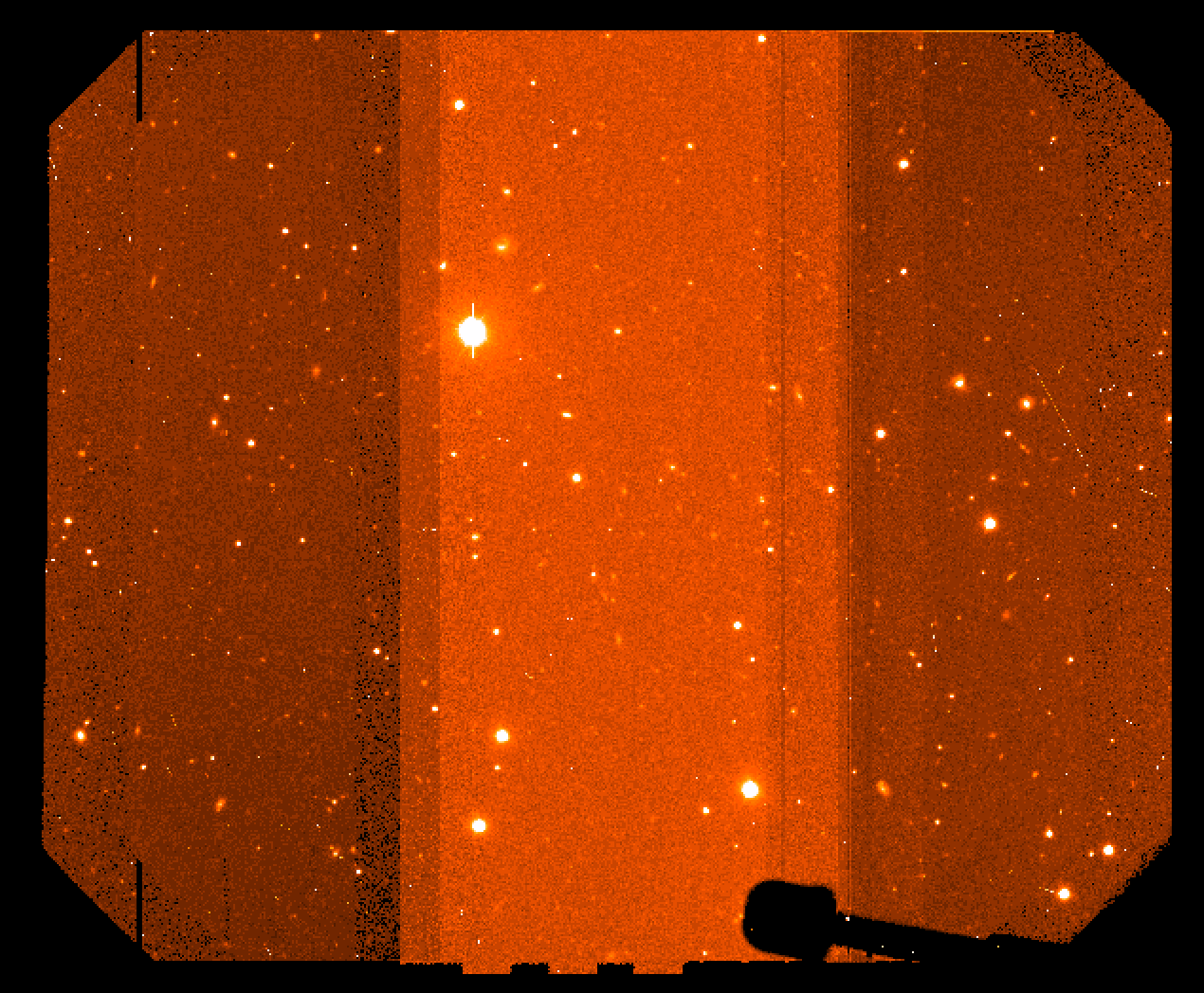
Figure 3: mosaiced combined image showing different background counts due to RQE differences

If this is the case, one can compute the needed adjustment (using the same script we used for the twilights in step 2.) and apply a second gqecor

files frqrg*.fits > qe_list.txt
cl < qemeasure_adv_YYYYMMMDD.cl
gqecorr @qe_list.txt logfile='gqecorr_sci.log' qecorr_data=./gmosQEfactors_mod_tw.dat
gmosaic qfrqrg*.fits fl_fixpix- fl_clean-

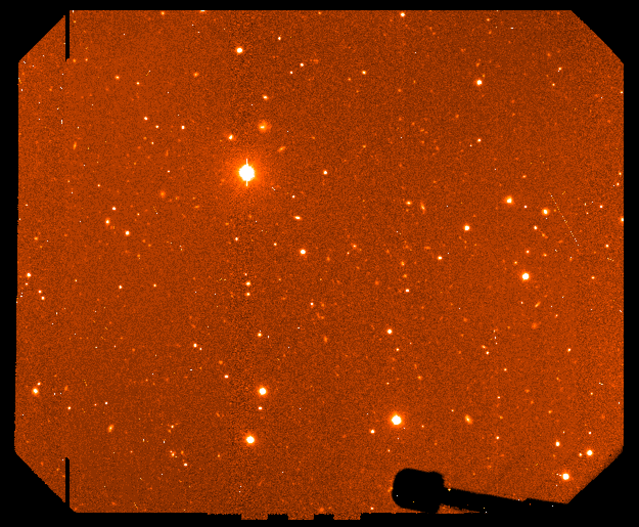
Figure 4: final mosaiced combined image.

8. Stack the mosaiced images:

This can be done either with imcoadd or gemcombine. In general I prefer the latter with median combining. When treating data affected by the amp#5 fault, this is the best option. Very important: for this to work fine, the lthreshold parameter must be adjusted to a positive value - but lower than the sky background (in this example the sky is at ~4100 counts). The purpose is to leave out amp5 (where all pixels are zero) from the median computation. Therefore, check the background level before running this.

gemcombine mqfrqrg*.fits output='median.fits' combine='median' reject='avsigclip' lthreshold=3800. offsets='wcs' scale='median'

(Or  mfrqrg*.fits if you did not apply the second gqecorr).

The scale='median' is necessary for a uniform background in the final image; in general the correction will be small. 

NOTE: the same exposure time is assumed for the individual images.

 9. Clean remaining Cosmic Rays (CRs):

This is an adaptation of the task crutil.crmedian for MEF fits.

crutil
imcopy median.fits[0] cmedian.fits[0]
crmedian median.fits[SCI,1] output='cmedian.fits[SCI,1]' crmask='bpm.fits' median=' '  sigma=' ' residual=' '  var0=0.  var1=0. var2=0. lsigma=100. hsigma=8. ncmed=5 nlmed=5 ncsig=15 nlsig=15

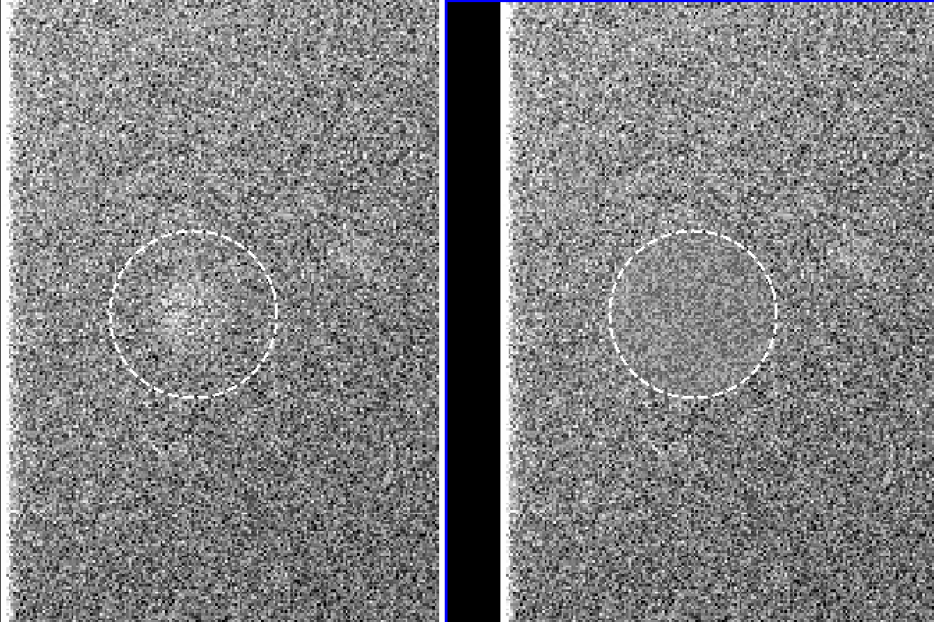
Lower "hsigma" parameter makes CR detection better, but too low can crop cores of bright stars or lines (see Fiigures 5 and 6).

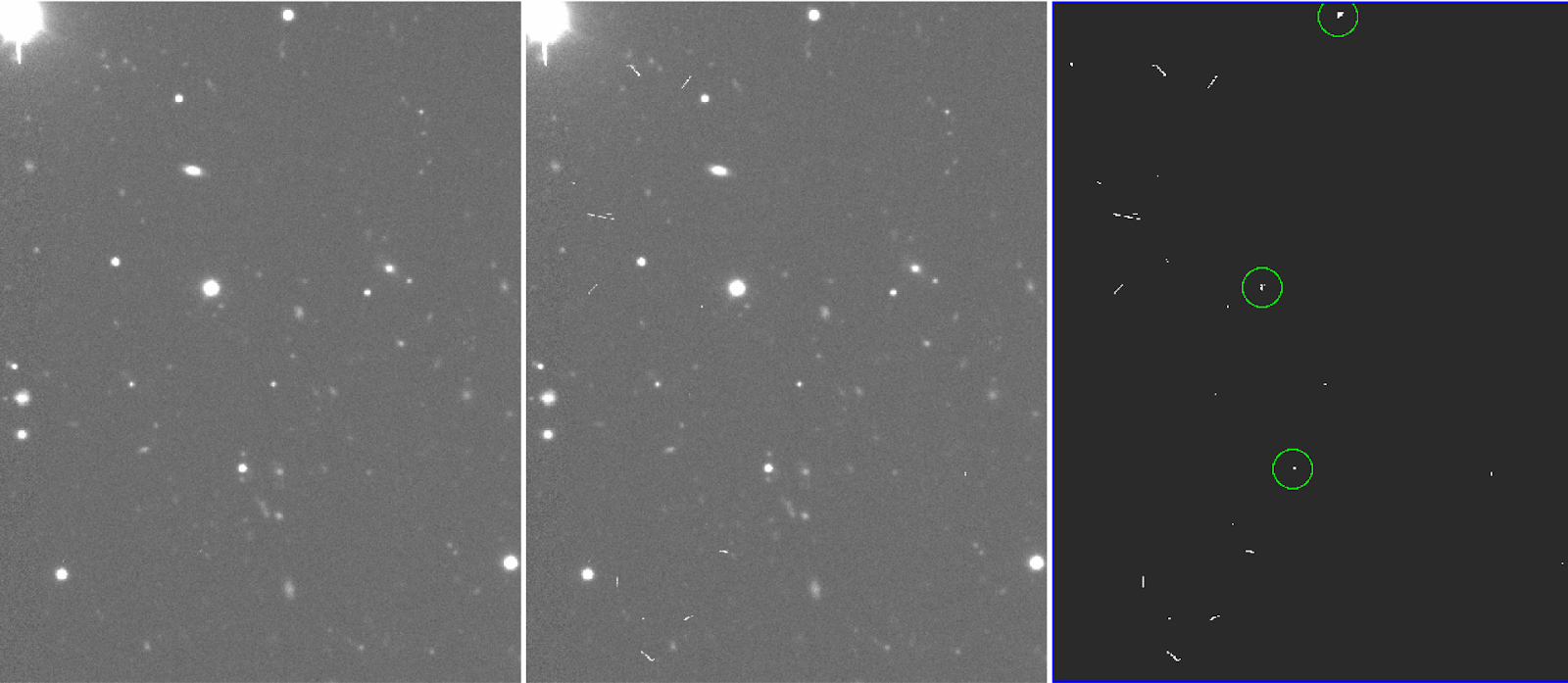
Figure 5: cleaned final image (left), original image (middle) and bpm (right), generated from the crmedian task. In this example (hsigma=6) masks the cores of some bright stars.

Figure 6: same as fig.5, but with hsigma=8. The cores of bright stars are not masked this time.

Generally this is a matter of trial and error, but hsigma=8 seemed to work fairly well in this case. By inspecting the bpm, one can check whether stars or regions of interest are masked.

displ bpm.fits[1] 1

Footnotes

[1] (1, 2, 3) Overscan order must be the same throughout the reduction process. A high order for the overscan fit provides better result across the FOV (except for the bottom ___ rows)

[2] (1, 2, 3) Bias must be overscan subtracted. The overscan fit order must be the same used in the science frames (be aware that processed bias available in the archive use the default order)

[3] (1, 2, 3) There are different bad columns masks depending on detector “flavor” . For the E2V detectors there is only 1 bad column on CCD2. For the Hamamatsu the bad columns changed over time (see masks list vs. time).

[4] (1, 2) It is important to note that the “scale” parameter within the task girmfringe may need to be adjusted in order to remove the fringing properly (by default the auto-scale algorithms within the task are used, however not always yield the optimal result).

[5] There are IRAF tasks that build illumination correction frames, however the results is not satisfactory within the whole GMOS FOV.

[6] Unfortunately, just building a median (e.g. with gemcombine) and using it for this doesn’t work quite well (in the sense there could be significant residuals remaining) Most times it is also necessary to mask the bright sources while constructing the median. Sometimes smoothing the median is also advisable.

[7] If there are negative residuals, then the masking and/or smoothing when construction the median flat needs to be improved.

Science longslit spectroscopy

Case 1: The correct way to use QE correction

Sometimes, after the reduction of the GMOS longslit spectroscopic data of the standard flux star, it is possible to see that the flux does not converge in the extremes of the CCD gaps, producing two artificial "steps” in the final spectrum. This problem propagates to all science frames as well.

Take in consideration that the gqecorr task generates two outputs:

1. qFlat_std.fits: quantum efficiency-corrected flat;

2. qecorrgs#name_arc.fits: this file (prefix “qecorr” + gs#name_arc.fits, which is the processed arc frame) is the QE correction image that needs to be used in the science frames.

When #QUANTUM-CORRECTING STANDARD STAR # it is run, specify the following:

gqecorr gs#name_Std.Star.fits refimage=gs#name_arc.fits corrimages=qecorrgs#name_arc.fits

Science MOS spectroscopy

Case 1: gswavelength crashes

When gswavelength task crashes on one of the slit lets, should hack gswavelength script at line 239 "loop over extensions”.

Case 2: Partial or full slit(s) blockage on MOS masks

1- Run gsflat on the gcalflat (any of them, for this purpose you need only one) with the options: fl_keep+ combflat="f_comb_whatever.fits"

gcalflat image001.fits image002.fits …  fl_keep+ combflat="f_comb_whatever.fits"

2- Run gsmosaic on the "f_comb_whatever.fits"

gsmosaic f_comb_whatever.fits

3- Hack gscut so it *does not* apply the slit length from the MDF, comment out the lines:

# y2 = y1 + specwid-1

# ry2 = ry1 + specwid-1

4- Run the hacked gscut on the mosaiced flat using itself as the gradient image.

Example:

gscut inimage=mf_comb_whatever.fits outimage=uumf_comb_whatever.fits gradimage= mf_comb_whatever.fits yoffset=82 

NOTE: mind the YOFFSET value. In the example, 82 worked OK. If the script has difficulties finding the slits then the YOFFSET may be off. Try varying this value and compare results.

5- Run gsreduce on the arc frames with fl_gmosaic+ fl_cut+ refimage=uumf_comb_whatever.fits outimage=uupOUTimage.fits

Example:

gsreduce uupINimage.fits fl_gmosaic+ fl_cut+ refimage=uumf_comb_whatever.fits outimges=uupOUTimage.fits 

If you gdisplay this arc (uupOUTimage.fits) you will see one of the extension without data.

6- Reassembling the MEF file by replacing the faulty one with a valid one, resulting in duplicate spectrum. The ggrebuild.cl script can be used for this. Consult the internal code for instructions. In the example, the extension [SCI, 34] is empty and will be replaced by [SCI, 33].

NOTE: ggrebuild.cl is also available to download from the Gemini Data Reduction forum http://drforum.gemini.edu/topic/wavelength-solutions-in-gmos-mos-spectra-script-to-fit-specific-sci-extensions/

7- Run gswaveleng on the rebuilt arc. The extension "n" is added

Example:

gswavelength inimages=nuupOUTimage.fits 

8- Run gstransform:

Example:

gstransform nuupOUTimage.fits wavtran=nuupOUTimage fl_inter- 

NOTE: remember which was the duplicated one.

Case 3: Wavelength Solutions: script to fit specific sci extensions

If in a particular slit of the arc frame where there is no visible line to be used to get the wavelength solution, the gswavelength task failing on this slit and subsequently fails on the rest of the slits.

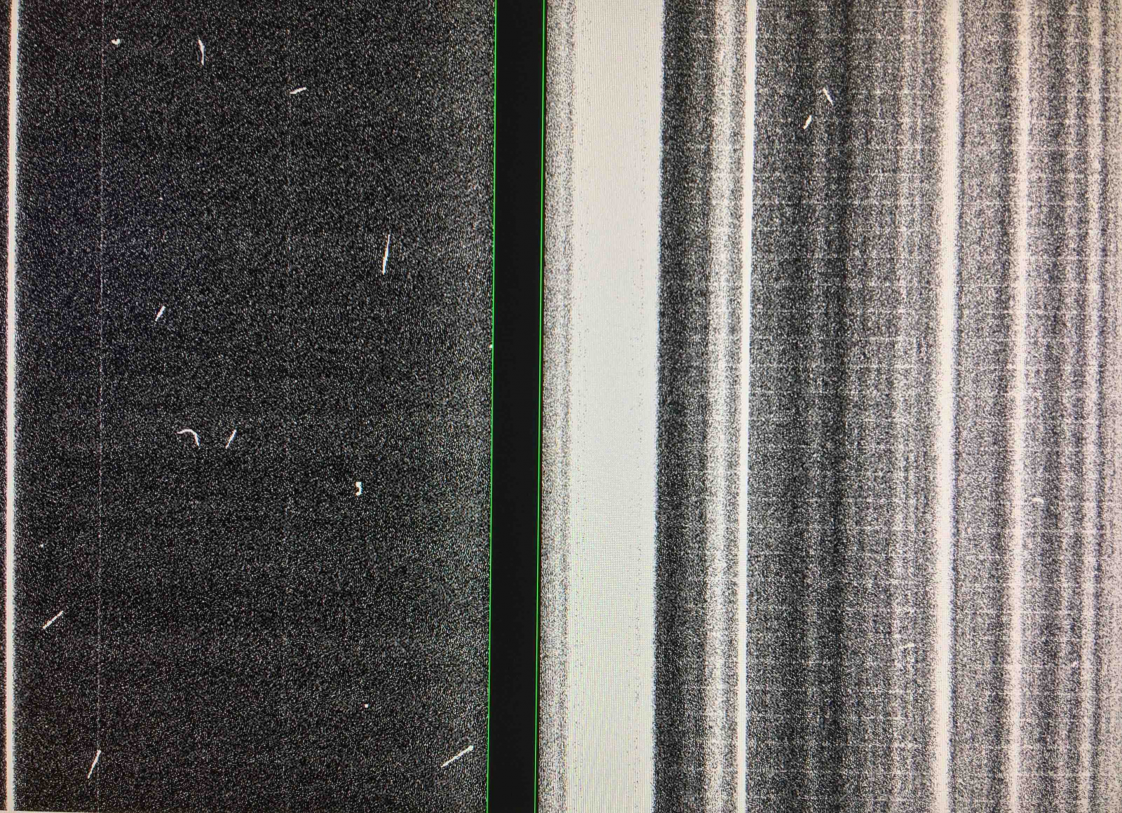
Example: On top, the extension [22] of the arc frame with signal, on bottom no signal on extension [23].

- Run the script mgswavelength.cl which allows to skip the problematic slit.

NOTE: mgswavelength.cl is also available to download from the Gemini Data Reduction forum, http://drforum.gemini.edu/topic/wavelength-solutions-in-gmos-mos-spectra-script-to-fit-specific-sci-extensions/

It allows the user to select the subset of extensions and in that way they can skip the slits that are causing the problem with the reduction process or getting the wavelength solution.

Case 4: Wavelength Calibration: autoidentify could not find solution

When autoidentify could not find solution during the Wavelength Calibration in GMOS MOS spectra:

-Run gswavelength task varying the "fwidth" parameter value and use order=4 and step=2.

gswavelength ugpS#.fits fl_inter- order=4 nlost=10 logfile="gswav_arc.log" step=2  fwidth=number 

If you use "fwidth" default value (fwidth=10), did not work either. However we found that using fwidth=3 autoidentify could find a solution.

gswavelength ugpS#.fits fl_inter- order=4 nlost=10 logfile="gswav_arc.log" step=2 fwidth=3.   

When the is a size mismatch error after running gstrasform:

- Use the option "refimage" for gscut with gsreduce task, setting as reference the arc frame; raten than using the MDF. This is implemented in the script red_mos_02.2020jun08.cl version.

NOTE: red_mos_02.2020jun08.cl is also available to download from the Gemini Data Reduction forum, http://drforum.gemini.edu/topic/wavelength-solutions-in-gmos-mos-spectra-script-to-fit-specific-sci-extensions/

Science 3D spectroscopy

coming soon

Appendix

A.1 Bad columns treatment (all modes) on “Hamamatsu/EEV” detectors

There are bad pixel masks (BPMs) that are used for masking the bad columns. From here on “BPM” will refer to this type of mask. The masks are multi-extension .fits frames, bad pixels have a value of 1 and good pixels are 0.

A.1.a) How to generate the BPM

• Given that the bad columns saturate after a few tens of seconds exposure time, the easiest way is to use the science data themselves for deriving the BPM. The simplest procedure is to make a copy of the science frame (and name it “mask.fits”  -do not edit the original!), replace by zero all values below a certain upper boundary (e.g. 60000), and then all the rest by 1. The IRAF task imreplace is particularly handy for this since in can be run directly over each extension:

imreplace ("mask.fits[1]", value=0. ,lower = INDEF, upper=50000.)  # set to zero anything below UPPER
imreplace ("mask.fits[1]", value=1. ,lower = 1., upper=INDEF)      # set to 1. all the rest
 …
 …    (continue with the rest of the extensions)

This works well in most cases, particularly spectroscopy in all modes. Of course if you have saturating objects those will be masked as “bad pixels” also with this procedure.

If you have three or more science exposures with the same binning and ROI (e.g. three spectra) it is better to median-combine them (e.g. with gemcombine) and perform the step above on the resulting median image.
Since the position of the bad columns is fixed, another alternative is to generate the BPM from the columns location and width in pixels (e.g. using IRAF tasks imexpr and imreplace).

Sometimes happens that after using the BPM (see next section) a residual bad column remains - this is due to the fact that  the bad columns generated this way (i.e. from the data) are still too narrow. The solution is to widen them (usually by 1-2 pixels is enough).

This example IRAF script ggbpm.02.2018feb07.cl generates a BPM from three images and performs the widening of the bad columns. Adjustable parameters are the upper limit for column detection (the bad columns are usually above 30k counts) and the width of the kernel for the widening function (1-2 pixels). These can be modified inside the code.

NOTE: ggbpm.02.2018feb07.cl is also available to download from the Gemini Data Reduction forum http://drforum.gemini.edu/topic/wavelength-solutions-in-gmos-mos-spectra-script-to-fit-specific-sci-extensions/

Once the mask is built, you need to inspect it visually in order to check whether there are any undesired features (e.g. bright object mistakenly considered as ‘bad pixels’). In case you find such features you can manually edit or remove them with the task imreplace.

A.1.b) How to use the BPM

• In order to use this MEF BPM for correcting the bad columns in an image, the script ggbpm.04.2018jun28.cl is needed. This is basically a wrapper that runs the task crfix over each extension of the image, and updates the OBJECT header keyword.

NOTE: ggbpm.04.2018jun28.cl is also available to download from the Gemini Data Reduction forum http://drforum.gemini.edu/topic/wavelength-solutions-in-gmos-mos-spectra-script-to-fit-specific-sci-extensions/

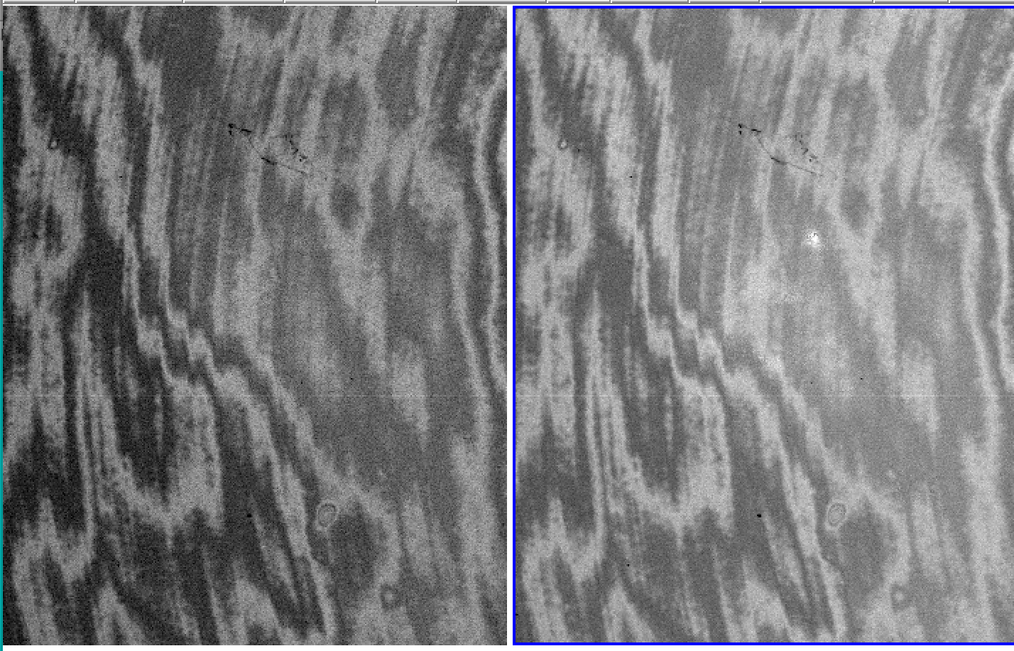
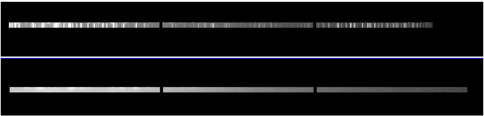
A.2 Amp5 bad column saturation banding problem

This affects only data taken while the Cboards were installed (2014jun01-2015sep01). Data is not destroyed by this, it is only a depression on the bias level. The main issue was that it varied with exposure time and over time also. To recover the correct shape, the most effective procedure is to work with extension 5 separately, mask any source signal on it in order to generate a flatfield.

In the example below from a spectroscopic longslit observation, the extension 5 shows the ‘banding’ effect arising from the saturation of the bad column (left panel). In the middle panel, we show the result of median-combining three exposures (note that for this to work you need to have at least three spatial-dithered exposures of the same exposure time). This can be used as a flatfield. The right panel shows the result of dividing the image on the left by the median shown in the middle.

In case you only have only one exposure, it would depend on the type of observation; but the idea is to interpolate the background across the affected area and build an ad-hoc flatfield image. The tasks imedit and fixpix are useful for this (see the example in item 6. of case 1.C)).

A.3 Biases structures

As a general rule, using biases closest to the observing time will be the safest approach. While bias structures are found to be very stable over long periods of time, there have been various instances where these have changed significantly as a result of changes/issues with the detector electronics.

Dates:

• May 2014 and before: EEV detectors 
• Jun 2014 - Aug 2015: Hamamatsu detectors with ARC47 rev. C video boards

• Sep 2015 - present: Hamamatsu detectors with ARC47 rev. E video boards:

a) Sep 2015 - Jun 2016: Normal 

b) Jul 2016 - Sep 2016: new bad columns (these remain till today, amps 3, 5, 8, 11), and mild bar-like vertical structures (a few counts above the mean bias level) on CCD2.

 
c) Oct 2016 - Feb 2017: strong (100-400 counts above bias) vertical fringes on CCD2 and CCD3, and horizontal 1-pix stripes across CCD2 and CCD3.

  
d) Mar 2017- Apr 2018: Normal

 
e) May 2018: same as c.
f) Jun 2018: bright structures are completely gone and readout noise is back to its nominal value (~4e-). The CTE is ok in the three chips and charge smearing is no longer present in CCD1.

Periods during which CCD1 had 'bad-CTE'
2018 April 15 - 2018 April 27
2018 May 14 - 2018 May 28 
2019 April 11 - 2019 June 24
2019 December 18 - 2020 March 14
2020 October 24 - 2021 April 05
NOTE: PIs with GMOS-S data observed during any of these periods are encouraged to assess whether this had a negative impact.

g) September 27th, 2021 to October 8th, 2021:  features enhanced noise structure in the detector amplifier#5 in CCD2.

h) February 10th, 2022:  re-appearance of the CTE problem on CCD1, plus high noise structure on CCD2. 

i) March 14th, 2022 to present: the CCD1 CTE issue was fixed, the noise problem on CCD2 and CCD1 persists.