Locations
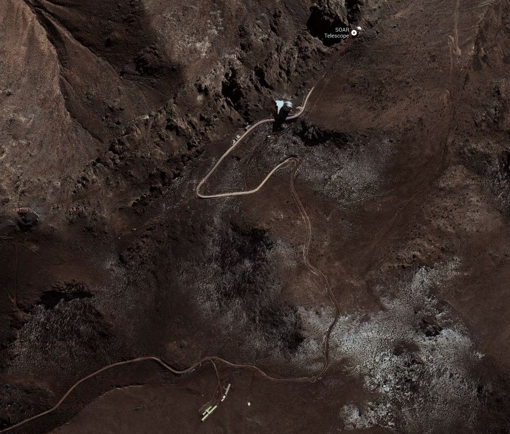
The Gemini South telescope is situated near the summit of Cerro Pachon in central Chile, at an altitude of 2722 m, at latitude -30:14:26.700 and longitude -70:44:12.096 in the WGS84 system.
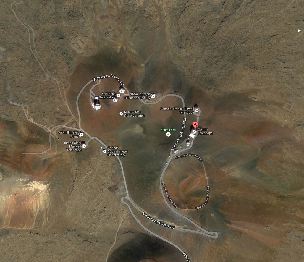
The Gemini North telescope is situated near the summit of Mauna Kea on the island of Hawaii, at an altitude of 4213 m, at latitude 19:49:25.7016 and longitude -155:28:08.616 in the WGS84 system, or at latitude 19:49:25.68521 and longitude -155:28:08.56831 in the NAD83 system (for a complete listing of Mauna Kea telescope coordinates on this system see here).
Google maps below show the telescope sites.
|
|
|
|
|
|
Observing Condition Constraints
![[weather icon]](/images/pio/20031125_LenticPanFlatII.jpg) All queue-mode observations must have observing condition constraints specified by the proposer that describe the minimum (i.e. poorest) conditions under which the observation should be executed. Classical programmes must also specify the minimum acceptable conditions and, optionally, a backup programme able to take advantage of poorer conditions. The observing condition constraints must be specified in the Phase I proposal to avoid loading the queue entirely with one type of condition (e.g., best image quality). See the Changing Details of Approved Programs web page for information on how to request a change to approved observing constraints or to add airmass or hour angle constraints.
All queue-mode observations must have observing condition constraints specified by the proposer that describe the minimum (i.e. poorest) conditions under which the observation should be executed. Classical programmes must also specify the minimum acceptable conditions and, optionally, a backup programme able to take advantage of poorer conditions. The observing condition constraints must be specified in the Phase I proposal to avoid loading the queue entirely with one type of condition (e.g., best image quality). See the Changing Details of Approved Programs web page for information on how to request a change to approved observing constraints or to add airmass or hour angle constraints.
The constraints are divided into five categories (if appropriate, values for Mauna Kea and Cerro Pachon are given separately):
- Image quality
- Sky transparency (cloud cover)
- Sky transparency (water vapor content)
- Sky background
- Airmass (zenith distance)
The first four of these are specified in the Phase I (initial) proposal; the airmass may be specified in the Observing Tool during Phase II.
Some of the specific properties corresponding to these categories are wavelength dependent and are not relevant for all observations. For example, the sky background at visible wavelengths is dominated by the lunar phase and moon-to-target angle, whereas at mid-IR wavelengths the combination of cloud cover and water vapour condition affect the background and its variability. For image quality, sky transparency and background we have chosen to represent the variation in these conditions (which is deterministic in the case of visible sky brightness, statistical in the case of quantities such as water vapour column) by a percentile representing the frequency of occurrence of the specific property. Observing constraints are specified in terms of these percentiles e.g. (best) 20%-ile, 50%-ile (better than median) etc.
This page provides a translation between the frequency of occurrence and the specific value for the relevant property as well as further information and guidance on their use by observers. The emphasis is on providing observers with these constraints in meaningful units (and corresponding to those used in the integration time calculators) as well as indicating their likelihood.
These examples illustrate some of the factors that a user might take into account when selecting their observing condition constraints:
- Example - NIRI spectroscopy of an extended object
- Example - NIRI imaging of structure within an extended object
More information about how observing conditions affect data quality is also available for the near-IR and mid-IR. In addition, (large ascii) files containing model high resolution spectra of the sky emission and transmission for a range of airmasses and water vapor columns are available for the near-IR and mid-IR.
Image Quality(non-AO) - MK and CP
CURRENT CONSTRAINTS (since 2014B)
| Wavelength regime | PSF FWHM at zenith (arcsec) | |||
| 20%-ile | 70%-ile | 85%-ile | "any" (100%-ile) | |
| u (0.350 µm)* | 0.60# | 0.90 | 1.20 | 2.0 |
| g (0.475 µm) | 0.60# | 0.85 | 1.10 | 1.90 |
| r (0.630 µm) | 0.50# | 0.75 | 1.05 | 1.80 |
| i (0.780 µm)* | 0.50# | 0.75 | 1.05 | 1.70 |
| Z (0.900 µm)* | 0.50# | 0.70 | 0.95 | 1.70 |
| Y (1.02 µm)* | 0.40 | 0.70 | 0.95 | 1.65 |
| J (1.2 µm) | 0.40 | 0.60 | 0.85 | 1.55 |
| H (1.65µm)* | 0.40 | 0.60 | 0.85 | 1.50 |
| K (2.2 µm) | 0.35 | 0.55 | 0.80 | 1.40 |
| L (3.4 µm) | 0.35 | 0.50 | 0.75 | 1.25 |
| M (4.8 µm)* | 0.35 | 0.50 | 0.70 | 1.15 |
| N' (11.7 µm filter) | 0.31-0.34 | 0.37 | 0.45 | 0.75 |
| Q (18.3 µm filter) | 0.49-0.54 | 0.49-0.54 | 0.49-0.54 | 0.85 |
Example interpretation of the table An image at K of a target at zenith would be expected to have a profile full width at half maximum of no more than 0.35 arcsec 20% of the time and no more than 0.55 arcsec 70% of the time.
# IQ20 bin limits for u, g, r, i, and Z were changed in 2014B based on IQ statistics from GMOS images as measured by the data quality assessment pipeline.
* Values for the marked bandpasses are interpolated or extrapolated from other values in the table. Note that the relevant parameter here is image quality and not simply seeing, that is, a wind speed distribution and the telescope performance (e.g. windshake and wavefront sensor performance) have been incorporated into the analysis.
Please read the following essential notes:
- Definition of values
Numerical values in the constraint columns are the current measured delivered image quality, defined as the Full Width at Half Maximum (FWHM) in arc-seconds, of the radial profile of the image of a point source at the zenith, measured from the science instrument detector at the specified wavelength. The FWHM is equal to the 50% Encircled Energy Diameter for a Gaussian profile, but is typically 30% larger than the FWHM for the GMOS PSF. The model was adapted by Mark Chun from original Mathematica calculations by Charles Jenkins (see also Jenkins 1998, MNRAS, 294, 69) with a subsequent correction (in August 2002) by Phil Puxley to the extant seeing distribution. - Determining the image quality at the start of an observation
The FWHM of the image of a point source (during acquisition), or when the adaptive optics wavefront sensor is used the image quality derived from its performance, is used to determine the initial image quality percentile band. - Determining the image quality during an observation
Monitoring of the image quality during observations uses science images or spectral cross cuts (if the spectrum is bright enough), or uses the image quality as measured by the wavefront sensor to track changes. In most, but not all cases (e.g., GNIRS in some modes) the image quality defined by the FWHM of a cross-cut through the spectrum is the same as the above. In all cases it is the measured or inferred "imaging image quality" that is used to specify the percentile band. In order to account for small variations in image quality during an observation, zenith-corrected image quality measurements that are less than 0.05 arcseconds higher than the limits in the tables above are considered to be acceptable. - Dependence on Telescope Elevation
The values in the above table apply to the telescope pointing at zenith. The FWHM percentile boundaries change (increase) with increasing airmass. The performance degradation away from the zenith can be approximated crudely as (airmass)0.6 in the visible and short wavelength infrared. Plots of the approximate delivered optical image quality as a function of airmass are given here. The integration time calculators take into account the dependence of image quality on wavelength (by interpolation) and airmass when calculating signal-to-noise ratios. The exponent is lower and variable in the 10 µm and 20 µm windows; values being used in the integration time calculators at these wavelengths are uncertain and may be updated. If your program requires a certain absolute image quality (e.g. for resolving objects at small separations) you should consider the possible elevations at which your observations could be executed when deciding upon image quality constraints. - Wavefront sensors
Use of wavefront sensors for image motion compensation (fast guiding) is required. For most wavelengths, values for peripheral and on-instrument WFSs are given (see each instrument's guiding options pages for details of available wavefront sensors). In all cases the use of a wavefront sensor for closed-loop primary mirror figure (AO) correction is assumed. - Mid-infrared
Image quality at Gemini South has been measured to be within ~10%(~20%)(~50%) of the theoretical diffraction limit 20%(70%)(85%) of the time in the 10 µm atmospheric window and within 10% of the diffraction limit 85% of the time in the 20 µm atmospheric window. The diffraction-limited FWHM is 0.31" at 11.7µm and 0.49" at 18.3 µm, the central wavelengths of the filters in which the percentiles have been evaluated. Similar values have been found at Gemini North. Note that there is little difference between the 20%-ile and 70%-ile image quality bins in the N band and no difference between 20%-ile, 70%-ile, and 85%-ile in the Q band. PIs may wish to take this into account before requesting IQ20 conditions given their low frequency of occurrence. - IQ = "Any"
This means that the observation can be scheduled under any image quality conditions. At optical and near-IR wavelength the image quality distribution has a long (non-Gaussian) tail. The values quoted are typical of the poorest conditions. - Adaptive Optics
Estimates of the AO-corrected image quality are described on the Altair pages.
Previous constraints (2014A and before)
| Wavelength regime | PSF FWHM at zenith (arcsec) | |||
| 20%-ile | 70%-ile | 85%-ile | "any" (100%-ile) | |
| U (0.365 µm)* | 0.50 | 0.90 | 1.20 | 2.0 |
| B (0.445 µm)* | 0.45 | 0.85 | 1.15 | 1.95 |
| V (0.5 µm) | 0.45 | 0.80 | 1.10 | 1.90 |
| R (0.658 µm) | 0.45 | 0.75 | 1.05 | 1.80 |
| I (0.806 µm)* | 0.40 | 0.75 | 1.05 | 1.70 |
| Z (0.900 µm)* | 0.40 | 0.70 | 0.95 | 1.70 |
| Y (1.02 µm)* | 0.40 | 0.70 | 0.95 | 1.65 |
| J (1.2 µm) | 0.40 | 0.60 | 0.85 | 1.55 |
| H (1.65µm)* | 0.40 | 0.60 | 0.85 | 1.50 |
| K (2.2 µm) | 0.35 | 0.55 | 0.80 | 1.40 |
| L (3.4 µm) | 0.35 | 0.50 | 0.75 | 1.25 |
| M (4.8 µm)* | 0.35 | 0.50 | 0.70 | 1.15 |
| N' (11.7 µm filter) | 0.31-0.34 | 0.37 | 0.45 | 0.75 |
| Q (18.3 µm filter) | 0.49-0.54 | 0.49-0.54 | 0.49-0.54 | 0.85 |
Cloud Cover - MK and CP
| Wavelength regime | Constraint and description | Comments | ||||
| 50%-ile | 70%-ile | 80%-ile | any | |||
| no signal loss | signal loss < 25% (0.3 mag) | 25% < signal loss < 60% (1 mag) | signal loss > 60% | |||
| optical | photometric | patchy cloud or extended thin cirrus | cloudy | usable | ||
| near-IR (1-2.5µm) | photometric | patchy cloud or extended thin cirrus | cloudy | usable | ||
| near-IR (3-5µm) | photometric | patchy cloud or extended thin cirrus | unusable except perhaps for VERY bright objects | not usable under 80% or poorer conditions due to emissivity | ||
| mid-IR (8-25µm) | cloudless | patchy cloud or extended thin cirrus | ||||
Explanation of table entries:
- The percentiles, which are based on long-term data for Mauna Kea, correspond to percentages of the time which have that transparency.
- "Photometric" - cloudless and capable of delivery of stable flux.
- "Cloudless" - for photometry accurate to a few percent in the mid-IR, careful attention must be paid to regular observations of suitable standard stars. The former 20%-ile ("low sky noise") bin was removed from this table as it proved impractical to measure.
- "Patchy cloud or extended thin cirrus" - relatively transparent patches, sometimes amongst thicker cloud resulting in some loss in transmission and variability, or a more uniform covering of thin cloud (usually cirrus). For the purpose of integration time calculation it is assumed that clearer patches have a transmission that is poorer by 0.3 mag than the nominal atmospheric extinction and that extended cirrus attenuates by no more that 0.3 mag (T~75%).
- "Cloudy" - cloud cover over essentially the whole sky. For the purpose of integration time calculation it is assumed that the transmission is poorer by 1 mag (T~40%) than the nominal atmospheric extinction and is variable. For semester 2011A and earlier this was a 90%-ile bin corresponding to 2 magnitudes of extinction (T~15%). The increase in background makes these conditions unusable at thermal infrared wavelengths, except perhaps for some very bright targets in high resolution spectroscopic modes. Stable guiding can be difficult in these conditions.
- "Usable" - any conditions under which the telescope is open. The increase in background makes these conditions unusable at thermal infrared wavelengths. For the purpose of integration time calculation it is assumed that the transmission is poorer by 3 mag (T~6%) than the nominal atmospheric extinction. Stable guiding can be difficult or impossible in these conditions.
Precipitable Water Vapor - MK and CP
Note that observations short of 1.3 microns are negligibly affected by water vapor. You should quote "Any" in your WV constraint. If you have a sky transparency (cloud cover) requirement, please refer to the section above.
| MK | Wavelength regime | Constraint (at zenith) | Comments | |||
| 20%-ile | 50%-ile | 80%-ile | any | |||
| optical | any | see note 2 | ||||
| near-IR (1-2.5µm) | 1.0mm | 1.6mm | 3mm | any | Precipitable H2O; primarily affects 1.35-1.50, 1.75-1.95, and 2.35-2.55 microns. See spectra. | |
| near-IR (3-5µm) | 1.0mm | 1.6mm | 3mm | any | Precipitable H2O; primarily affects 2.80-3.25 and 4.8-5.5 microns. See spectra. | |
| mid-IR (8-25µm) | 1.0mm | 1.6mm | 3mm | any | Precipitable H2O; primarily affects 7-8, 12-14, and 17-25 microns. See spectra. | |
Note that Cerro Pachón does not currently have the capability to measure the atmospheric water vapor content. Hence for the Gemini-South telescope observing constraints on water vapor cannot be guaranteed and it is recommended that they be set to WV/Any to avoid confusion.
| CP | Wavelength regime | Constraint (at zenith) | Comments | |||
| 20%-ile | 50%-ile | 80%-ile | any | |||
| optical | any | see note 2 | ||||
| near-IR (1-2.5µm) | 2.3mm | 4.3mm | 7.6mm | any | Precipitable H2O; primarily affects 1.35-1.50, 1.75-1.95, 2.35-2.55 microns. See spectra | |
| near-IR (3-5µm) | 2.3mm | 4.3mm | 7.6mm | any | Precipitable H2O; primarily affects 2.80-3.25 and 4.8-5.5 microns. See spectra. | |
| mid-IR (8-25µm) | 2.3mm | 4.3mm | 7.6mm | any | Precipitable H2O; primarily affects 7-8, 12-14, and 17-25 microns. See spectra. | |
Explanation of table entries:
- The values in the above table apply to the telescope pointing at zenith. The column of water along the line of sight scales linearly with the airmass, so strict constraints on the water vapor may need to be accompanied by constraints on the airmass.
- In the integration time calculators the optical transparency is derived from model transmission spectra. See "Sky Transparency (cloud cover)" for a related constraint.
- The atmospheric transmission is strongly wavelength dependent as shown in model transmission spectra. With the exception of water vapor the major absorbing species at infrared wavelengths (e.g/., CO, CO2, N2O, CH4, O3) have absorbing columns that depend only on airmass. However, the water vapor abundance above Mauna Kea and Cerro Pachon can vary by over an order of magnitude, even for clear skies. At many wavelengths in the near- and mid-IR transparencies are strongly dependent on the precipitable water vapor.The CSO 225 GHz optical depth, "tau", is used to determine the current PWV conditions on MK, using the conversion formula tau(225GHz) = 0.04 * mm(H2O) + 0.017 (Dempsey et al. 2013 MNRAS, 430, 2534). On CP the water vapour column is estimated from the Universidad de Chile Cerro Pachon forecast.
- Percentiles for Mauna Kea are based on long-term data. For Cerro Pachon, conditions are assumed to be similar to La Silla, where statistics indicate that the PWV is approximately twice that of Cerro Paranal. Therefore, the percentiles given are based on 1992-1994 data from the ESO/VLT site at Cerro Paranal, multiplied by 2. Note that the percentiles are based on year-round data, but the PWV during Chilean summer (Jan-Mar) is generally double that of the rest of the year, as shown in the Paranal data and the data from the ALMA site. The Mauna Kea data do not show a strong seasonal variation.
- "Any" means that the observation can be scheduled under any conditions.
Sky Background
| MK | Wavelength regime | Constraint (Vega mags) | Comments | |||
| 20%-ile | 50%-ile | 80%-ile | any | |||
| optical | µV > 21.3 ('darkest') |
µV > 20.7 ('dark') |
µV > 19.5 ('grey') |
µV > 18.0 ('bright') |
V-band mag/sq arcsec; sky color is different for each bin | |
| near-IR (1-2.5µm) | any J~16.1, H~13.8, K~14.8 |
brightness in mag/sq arcsec; see note 1 | ||||
| near-IR (3-5µm) | any | see note 2 | ||||
| mid-IR (8-25µm) | any | see note 2 | ||||
| CP | Wavelength regime | Constraint (Vega mags) | Comments | |||
| 20%-ile | 50%-ile | 80%-ile | any | |||
| optical | µV > 21.3 ('darkest') |
µV > 20.7 ('dark') |
µV > 19.5 ('grey') |
µV > 18.0 ('bright') |
V-band mag/sq arcsec; sky color is different for each bin | |
| near-IR (1-2.5µm) | any J~16.2, H~13.8, K~14.6 |
brightness in mag/sq arcsec; see note 1 | ||||
| near-IR (3-5µm) | any | see note 2 | ||||
| mid-IR (8-25µm) | any | see note 2 | ||||
Explanation of table entries:
- The near-infrared J- and H-band backgrounds are dominated by OH airglow lines. The K-band background has significant contributions from both OH and thermal emission from CH4 and H2O. Within the integration time calculator the OH background is assumed to be constant and only a function of airmass (once the sun is sufficiently below the horizon) even though the OH emission is known to vary during the night (more details).
- The near-IR 3-5 um and mid-IR 8-25 um backgrounds are determined by the (wavelength) dependent thermal emission from numerous atmospheric species including water vapour. Note that cloud cover conditions (which are defined in the Sky Transparency constraint) contribute to the infrared sky brightness, but are not part of this constraint).
- All values pertain to the zenith and 50%-ile H2O, and do not include telescope and instrument emission.
- Optical background values originate from a Monte Carlo simulation of the sky brightness using a model which includes scattered moonlight and zodiacal light, and pertains to high ecliptic latitude. The sky color is different between constraint bins. Crudely speaking, the moon is below the horizon during about one half of queue-mode hours. These tabulated values are used to scale an empirical sky spectrum within the integration time calculator.
- "Any" means that the observation can be scheduled under any (clear) sky background conditions.
Airglow
For information about how the airglow at Maunakea affects the Sky Background (at Gemini North) as a function of the time of the night, the Moon, the airmass or the season, see the page about Measurements of airglow on Maunakea (will open a new page from the GMOS instrument).
Airmass
This constraint defines the maximum airmass [= sec(zenith distance) =1/cos(zd)] at which the target should be observed. The airmass affects the sky transparency (e.g. the general atmospheric extinction as well as the depth and breadth of specific absorption bands due to atmospheric constituents such as H2O, CO, and CO2),sky brightness and image quality. As a crude first approximation, the sky transparency decreases and brightness increases in proportion to the increase in airmass (e.g. sky brightness is twice as great at airmass = 2 than at airmass = 1) and the optical image quality degrades as (airmass)0.6.
The airmass constraint is not used at Phase I, although it can/should be entered in the integration time calculators to make an accurate estimate of observing time and to show how the expected signal-to-noise for an observation varies with elevation. Elevation constraints can be inserted at Phase II. Note that the phase II default is no elevation constraint and any changes to the airmass or hour angle constraints require approval of the appropriate Head of Science Operations. An example of an observation that would use these constraints is one using GMOS that needs to restrict the hour angles so that the position angle of the slit(s) is close to the parallactic angle. Targets with no elevation constraints will be observed at airmasses less than 2.0.
Optical Sky Background
The optical sky background depends on a number of parameters including the target - moon angular separation, lunar phase, ecliptic latitude, zenith angle, and phase of the solar cycle (e.g. Krisciunas 1997, PASP, 209, 1181; Krisciunas and Schaefer 1991, PASP, 103, 1033; Benn and Ellison 1998, La Palma Technical Note 115). A model was constructed following the prescription of Krisciunas (1997) and Krisciunas and Schaefer (1991).
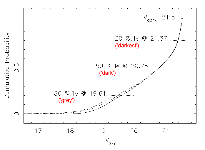
The graph below shows the cumulative probability distributions of V-band sky brightness at an arbitrary phase in the solar cycle for three model observation scenarios. In the first model the target is always at the zenith. The second and third models are more realistic Monte Carlo realisations of likely queue and classical programs. In the second model targets were chosen with a gaussian distribution in Hour Angle with sigma=1 hour, and with a distribution in Declination between -20 and +90 degrees based on the surface area of the celestial sphere. The third model is the same as the second, but with the further constraint that the target must be at least 30 degrees from the moon. It may seem surprising that the results of these 3 models differ so little. This is due to the fact that the primary dependence of night sky brightness is on lunar phase, and secondarily on moon - target distance.
The results of these calculations indicate that the sky at Mauna Kea is fainter than 20.78 mag/arcsec2 for 50% of the time and fainter than 21.37 mag/arcsec2 for 20% of the time for any random target. (For an unbiased distribution of queue-mode nights the moon is below the horizon for about half the time, of course).
The values presented in the observing constraints table are modified slightly each year or so to account for the nominal solar cycle variation.
The colour of the sky changes with lunar phase. Adopted values are shown in the table below (taken from ESO, by scaling V for inferred equivalent lunar phase, and from Walker, NOAO Newsletter No. 10). The conversion between the sky background category and the number of nights from new moon indicates the constraints that are applied to schedule classical observations and do not necessarily correspond to conventional definitions of dark, grey and bright time.
| Sky Background Category | Approx Nights From New Moon (+/-) | Sky Brightness (mag/arcsec2) | |||
| V-band | U-band | B-band | R-band | ||
| 20%-ile ('darkest') |
=< 3 | 21.3 | V + 0.0 | V + 0.8 | V - 0.9 |
| 50%-ile ('dark') |
=< 7 | 20.7 | V - 1.5 | V + 0.2 | V - 0.8 |
| 80%-ile ('grey') |
=< 11 | 19.5 | V - 2.2 | V - 0.0 | V - 0.4 |
| any ('bright') |
=< 14 | 18.0 | V - 3.0 | V - 0.5 | V - 0.1 |
Note that the V-band sky is brighter at low ecliptic latitude by ~0.4 mag (Benn and Ellison 1998. La Palma Technical Note 115).
Data from HM Nautical Almanac Office, showing sun and moon rising and setting times and lunar phases for Mauna Kea and Cerro Pachon/Tololo/La Silla can be found here.
The broad-band sky brightnesses given in the table above have been used to scaled a model optical sky spectrum . These spectra are used in the Integration Time Calculators. The sky spectrum is patched to the near-IR sky spectrum at a wavelength of 920nm. An example is shown below (for 50%, 'dark' conditions) and the data file is available.
Airglow
For information about how the airglow at Maunakea affects the Sky Background (at Gemini North) as a function of the time of the night, the Moon, the airmass or the season, see the page about Measurements of airglow on Maunakea (will open a new page from the GMOS instrument).
IR Sky Background
This page discusses the infrared sky background on Mauna Kea and Cerro Pachon. Files of sky emission spectra for the two sites are available at the bottom of the page.
Mauna Kea
The Mauna Kea sky background is described here for the following wavelength regimes:
The near-IR (1-2.5µm) sky background is dominated by many intrinsically narrow hydroxyl (OH) emission lines. A few other species (e.g. molecular oxygen at 1.27µm) also contribute, as do H2O lines at the long wavelength end of the K window. During the night the hydroxyl lines vary in brightness on a timescale of 5-15 minutes and with an amplitude of 5-10% as atmospheric wave phenomena change the local density of species. As the emission occurs via a radiative cascade, all of the lines vary together in brightness to first order.
The strength of the OH lines also exhibits a steady decline for the first 1-2 hrs after sunset. Spectroscopic observations at low and intermediate resolutions are usually not advisable during twilight, especially in the J and H bands, as it can be difficult to achieve accurate sky subtraction. Imaging observations of bright objects are possible, albeit with an increased and varying background.
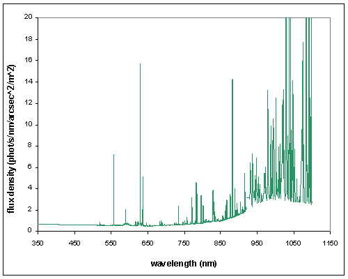
The IR Integration Time Calculators employ model high resolution sky emission spectra, an example of which is shown below. In addition to the OH lines, the models incorporate zodiacal continuum emission (approximated by a 5800K black body) (each then scaled by the atmospheric transmission), and thermal emission from the atmosphere (treated as a 273K black body for Mauna Kea and a 280 K blackbody for Cerro Pachon multiplied by 1 - transmission), at a variety of airmasses and water vapor columns. Note that moonlight, which is not included can be the dominant background source (e.g., much more so than in the model spectra), especially in the J band when the moon is bright and especially when the target is close to the moon.
For information about how the airglow at Maunakea affects the broadband Sky Background (at Gemini North in the J, H, K, and other windows) as a function of the time of the night, the Moon, the airmass or the season, see the page about Measurements of airglow on Maunakea (will open a new page from the GMOS instrument).
The near-IR (3-5µm) sky background is due primarily to thermal emission from the atmosphere. The transmission (and therefore the emission) varies with atmospheric water vapour content and air mass. See the descriptions of atmospheric transmission and the adopted water vapour conditions for more information. An example model background spectrum, smoothed to a resolution of 2cm-1, is shown below.
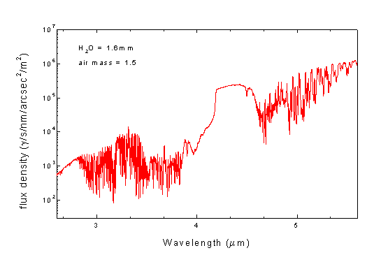
The mid-IR (7-25µm) sky background behaves similarly to the 3-5µm background, but is much more intense. See the descriptions of atmospheric transmission and the adopted water vapour conditions for more information.
Cerro Pachon
The sky background has been modeled for Cerro Pachon as well and is used in its ITCs. Data files are similar to those for Mauna Kea.
Sky Background Data Files
Raw sky emission data files 0.9-5.6 and 7-26 microns for both Mauna Kea and Cerro Pachon are available in ascii format via the following tables. These files are sky background only; they do not include the emission from the telescope itself and from the instrument (both of which are included in the IR Integration Time Calculators).
The files were manufactured starting from the sky transmission files generated by ATRAN (Lord, S. D., 1992, NASA Technical Memorandum 103957). These files were subtracted from unity to give an emissivity and then multiplied by a blackbody function of temperature 273 for Mauna Kea and 280 for Cerro Pachon. To these were added the OH emission spectrum (available from the European Southern Observatory's ISAAC web pages) a set of O2 lines near 1.3 microns with estimated strengths based on observations at Mauna Kea, and the dark sky continuum (in part zodiacal light), approximated as a 5800K gray body times the atmospheric transmission and scaled to produce 18.2 mag/arcsec^2 in the H band, as observed on Mauna Kea by Maihara et al. (1993 PASP, 105, 940).
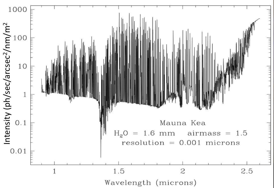
Any use of the data in these tables should reference Lord (1992) and acknowledge Gemini Observatory. The 1-5 micron models are in ASCII two-column format: (a) wavelength with a sampling of 0.00002µm and a resolution of 0.00004µm (0.04nm) and (b) emission in ph/sec/arcsec^2/nm/m^2 . The 7-26 micron models have a sampling of 0.0001µm and a resolution of 0.0002µm (0.2nm) for Mauna Kea and 0.002µm and 0.004µm (4nm) for Cerro Pachon.
Note the crudity of the approximation of the thermal background, which assumes that all sources of sky opacity are at T=273K on Mauna Kea and T=280 on Cerro Pachon. In reality the sources occur at various altitudes above each site. Thus, these files should overestimate the thermal background. Note also that the OH lines can vary in intensity from night to night and vary greatly during the night as well. Finally note that background from moonlight is not included, but it can be very significant in the J, H, and K bands, especially if the target is located close to the bright moon
(In most browsers, hold down the shift key when clicking to save the data to a file). The numbers in the titles of the files are 10X the water vapor in mm and 10X the airmass.
| Mauna Kea Sky Emission (0.9-5.6 microns) | |||||
| air mass | water vapor column | ||||
| 1.0mm | 1.6mm | 3.0mm | 5.0mm | ||
| 1.0 | mk_skybg_zm_10_10_ph.dat | mk_skybg_zm_16_10_ph.dat | mk_skybg_zm_30_10_ph.dat | mk_skybg_zm_50_10_ph.dat | |
| 1.5 | mk_skybg_zm_10_15_ph.dat | mk_skybg_zm_16_15_ph.dat | mk_skybg_zm_30_15_ph.dat | mk_skybg_zm_50_15_ph.dat | |
| 2.0 | mk_skybg_zm_10_20_ph.dat | mk_skybg_zm_16_20_ph.dat | mk_skybg_zm_30_20_ph.dat | mk_skybg_zm_50_20_ph.dat | |
| Cerro Pachon Sky Emission (0.9-5.6 microns) | |||||
| air mass | water vapor column | ||||
| 2.3mm | 4.3mm | 7.6mm | 10.0mm | ||
| 1.0 | cp_skybg_zm_23_10_ph.dat | cp_skybg_zm_43_10_ph.dat | cp_skybg_zm_76_10_ph.dat | cp_skybg_zm_100_10_ph.dat | |
| 1.5 | cp_skybg_zm_23_15_ph.dat | cp_skybg_zm_43_15_ph.dat | cp_skybg_zm_76_15_ph.dat | cp_skybg_zm_100_15_ph.dat | |
| 2.0 | cp_skybg_zm_23_20_ph.dat | cp_skybg_zm_43_20_ph.dat | cp_skybg_zm_76_20_ph.dat | cp_skybg_zm_100_20_ph.dat | |
| Mauna Kea Sky Emission (7-26 microns) | |||||
| air mass | water vapor column | ||||
| 1.0mm | 1.6mm | 3.0mm | 5.0mm | ||
| 1.0 | mk_skybg_nq_10_10_ph.dat | mk_skybg_nq_16_10_ph.dat | mk_skybg_nq_30_10_ph.dat | mk_skybg_nq_50_10_ph.dat | |
| 1.5 | mk_skybg_nq_10_15_ph.dat | mk_skybg_nq_16_15_ph.dat | mk_skybg_nq_30_15_ph.dat | mk_skybg_nq_50_15_ph.dat | |
| 2.0 | mk_skybg_nq_10_20_ph.dat | mk_skybg_nq_16_20_ph.dat | mk_skybg_nq_30_20_ph.dat | mk_skybg_nq_50_20_ph.dat | |
| Cerro Pachon Sky Emission (7-26 microns) | |||||
| air mass | water vapor column | ||||
| 2.3mm | 4.3mm | 7.6mm | 10.0mm | ||
| 1.0 | cp_skybg_nq_23_10_ph.dat | cp_skybg_nq_43_10_ph.dat | cp_skybg_nq_76_10_ph.dat | cp_skybg_nq_100_10_ph.dat | |
| 1.5 | cp_skybg_nq_23_15_ph.dat | cp_skybg_nq_43_15_ph.dat | cp_skybg_nq_76_15_ph.dat | cp_skybg_nq_100_15_ph.dat | |
| 2.0 | cp_skybg_nq_23_20_ph.dat | cp_skybg_nq_43_20_ph.dat | cp_skybg_nq_76_20_ph.dat | cp_skybg_nq_100_20_ph.dat | |
IR Transmission Spectra
The infrared spectra of the atmospheric transmission above Mauna Kea and Cerro Pachon that are used in the Integration Time Calculators have been generated using the ATRAN modelling software (Lord, S.D. 1992, NASA Technical Memor. 103957) and are presented separately for the near-IR and mid-IR. Ascii data files of these spectra are available below.
Near-IR
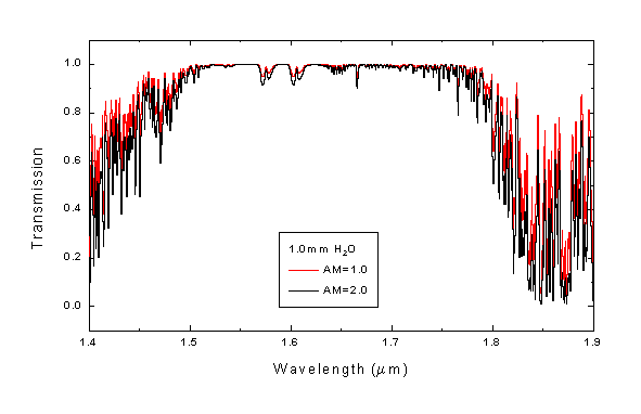
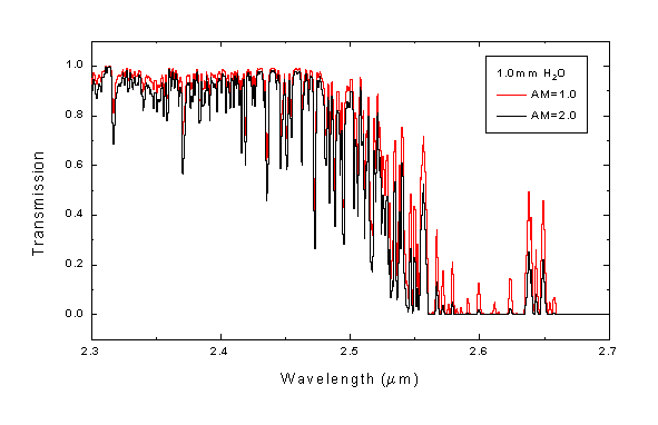
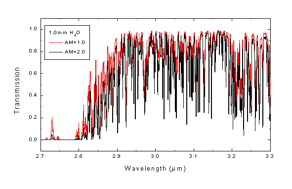
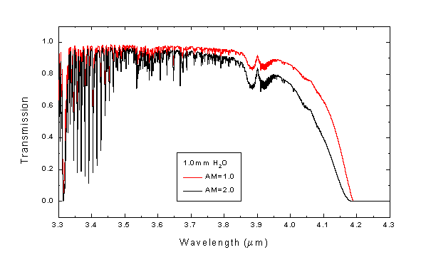
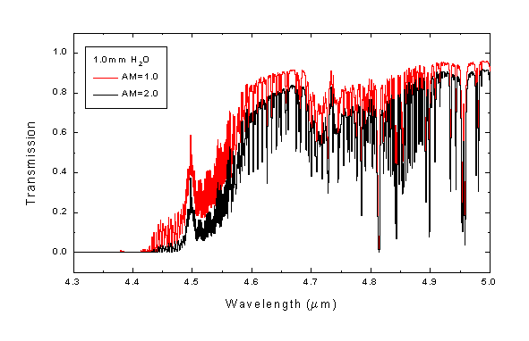
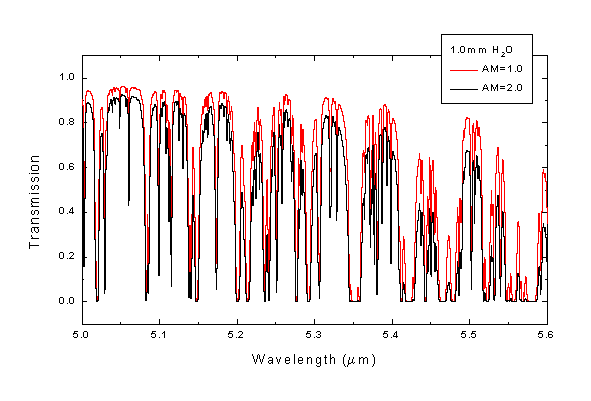
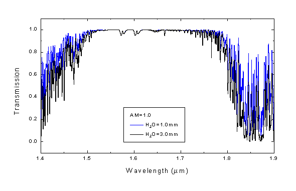
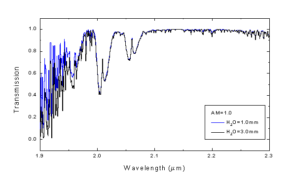
Overview spectra for Mauna Kea are presented below for the wavelength ranges 0.9 - 2.7 and 2.7 - 5.6µm with a water vapour column of 1.6mm and an air mass of 1.0. To assess appropriate observing condition constraints, the effects of water vapour and air mass can be examined on an expanded wavelength scale by clicking on the upper (red) or lower (blue) bars in the images. Doing so will show examples corresponding to (blue bar) 1.0 and 3.0mm precipitable water vapour at AM=1.0 and (red bar) AM=1.0 and 2.0 at 1.0mm H2O.
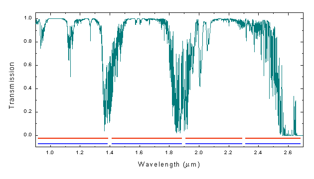
If image maps are not supported by your browser the expanded spectra may be displayed by selecting the appropriate wavelength range:
 AM=1.0 and 2.0 at 1.0mm precipitable water vapour: 0.9 - 1.4, 1.4 - 1.9, 1.9 - 2.3, 2.3 - 2.7, 2.7 - 3.3, 3.3 - 4.3, 4.3 - 5.0 and 5.0 - 5.6µm
 1.0 and 3.0mm H2O at AM=1.0: 0.9 - 1.4, 1.4 - 1.9, 1.9 - 2.3, 2.3 - 2.7, 2.7 - 3.3, 3.3 - 4.3, 4.3 - 5.0 and 5.0 - 5.6µm
The raw data files generated by ATRAN for 0.9-5.6 microns are available via the following table. Any use of these data should reference Lord, S. D., 1992, NASA Technical Memorandum 103957, and acknowledge Gemini Observatory. The models are in ASCII two-column format: (a) wavelength with a sampling of 0.00002µm and a resolution of 0.00004µm (0.04nm) and (b) transmission.(In most browsers, hold down the shift key when clicking to save the data to a file). The numbers in the titles of the files are 10X the water vapor in mm and 10X the airmass.
| Mauna Kea Sky Transmission (0.9-5.6 microns) | |||||
| air mass | water vapor column | ||||
| 1.0mm | 1.6mm | 3.0mm | 5.0mm | ||
| 1.0 | mktrans_zm_10_10.dat | mktrans_zm_16_10.dat | mktrans_zm_30_10.dat | mktrans_zm_50_10.dat | |
| 1.5 | mktrans_zm_10_15.dat | mktrans_zm_16_15.dat | mktrans_zm_30_15.dat | mktrans_zm_50_15.dat | |
| 2.0 | mktrans_zm_10_20.dat | mktrans_zm_16_20.dat | mktrans_zm_30_20.dat | mktrans_zm_50_20.dat | |
| Cerro Pachon Sky Transmission (0.9-5.6 microns) | |||||
| air mass | water vapor column | ||||
| 2.3mm | 4.3mm | 7.6mm | 10.0mm | ||
| 1.0 | cptrans_zm_23_10.dat | cptrans_zm_43_10.dat | cptrans_zm_76_10.dat | cptrans_zm_100_10.dat | |
| 1.5 | cptrans_zm_23_15.dat | cptrans_zm_43_15.dat | cptrans_zm_76_15.dat | cptrans_zm_100_15.dat | |
| 2.0 | cptrans_zm_23_20.dat | cptrans_zm_43_20.dat | cptrans_zm_76_20.dat | cptrans_zm_100_20.dat | |
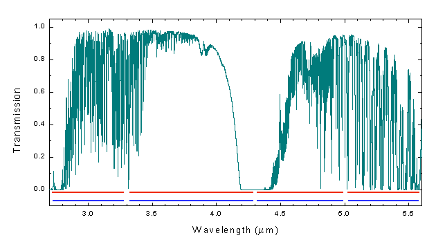
Mid-IR
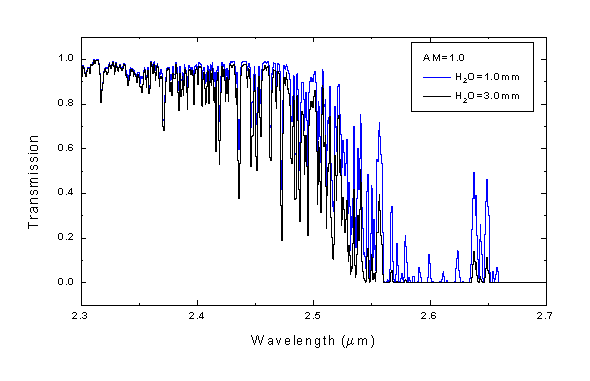
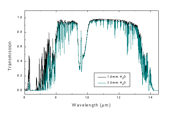
The atmospheric absorption in the 10µm-window is affected mainly by CO2, CH4, H2O and O3. The principal effect of an increase in the water vapour column above the site is an overall reduction of transmission, and consequent increase in the sky background, as shown by the curves for 1.0 and 3.0mm of H2O in the following figure:
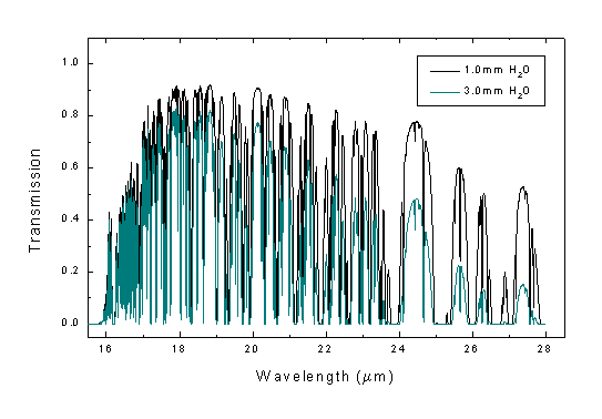
The far greater atmospheric absorption in the 20µm window is dominated by water vapour, as shown by the curves for 1.0 and 3.0mm of H2O in the following figure:
The raw data files generated by ATRAN for 7-26 microns are available via the following tables. Use of these data should reference Lord (1992) and acknowledge Gemini Observatory. The models are in ASCII two-column format: (a) wavelength with a sampling of 0.0001µm and a resolution of 0.0002µm (0.2nm) for Mauna Kea and 0.002µm and 0.004µm (4nm) for Cerro Pachon and (b) transmission.(In most browsers, hold down the shift key when clicking to save the data to a file). The numbers in the titles of the files are 10X the water vapor in mm and 10X the airmass.
| Mauna Kea Sky Transmission (7-26 microns) | |||||
| air mass | water vapor column | ||||
| 1.0mm | 1.6mm | 3.0mm | 5.0mm | ||
| 1.0 | mktrans_nq_10_10.dat | mktrans_nq_16_10.dat | mktrans_nq_30_10.dat | mktrans_nq_50_10.dat | |
| 1.5 | mktrans_nq_10_15.dat | mktrans_nq_16_15.dat | mktrans_nq_30_15.dat | mktrans_nq_50_15.dat | |
| 2.0 | mktrans_nq_10_20.dat | mktrans_nq_16_20.dat | mktrans_nq_30_20.dat | mktrans_nq_50_20.dat | |
| Cerro Pachon Sky Transmission (7-26 microns) | |||||
| air mass | water vapor column | ||||
| 2.3mm | 4.3mm | 7.6mm | 10.0mm | ||
| 1.0 | cptrans_nq_23_10.dat | cptrans_nq_43_10.dat | cptrans_nq_76_10.dat | cptrans_nq_100_10.dat | |
| 1.5 | cptrans_nq_23_15.dat | cptrans_nq_43_15.dat | cptrans_nq_76_15.dat | cptrans_nq_100_15.dat | |
| 2.0 | cptrans_nq_23_20.dat | cptrans_nq_43_20.dat | cptrans_nq_76_20.dat | cptrans_nq_100_20.dat | |
Sky Transparency/Extinction
The sky transparency is presented separately for Mauna Kea and Cerro Pachon.
Mauna Kea
The Mauna Kea sky transparency is described here for the following wavelength regimes:
The optical extinctions used in the Integration Time Calculators are model spectra that include scattering and absorption by water vapour and other atmospheric constituents.
For reference purposes only, median extinction coefficients for Mauna Kea are shown in the following table (Boulade 1988, CFHT Bulletin, 19, 16, for l<400nm; CFHT Observers Manual for l>400nm). They are insensitive to water vapour content.
| Wavelength (nm) | Extinction (mag / air mass) |
| 310 | 1.37 |
| 320 | 0.82 |
| 340 | 0.51 |
| 360 | 0.37 |
| 380 | 0.30 |
| 400 | 0.25 |
| 450 | 0.17 |
| 500 | 0.13 |
| 550 | 0.12 |
| 600 | 0.11 |
| 650 | 0.11 |
| 700 | 0.10 |
| 800 | 0.07 |
| 900 | 0.05 |
The near-infrared J, H and K wavebands are separated by regions of deep absorption predominantly due to water vapour. Transmission spectra were generated using the ATRAN model (Lord, S.D. 1992, NASA Technical Memor. 103957) for the adopted water vapour conditions (1.0, 1.6 and 3.0mm) at 1.0, 1.5 and 2.0 air masses. These spectra are used in the integration time calculators.
For reference purposes only, mean extinctions through broad-band filters for Mauna Kea are shown in the table below for 2mm of precipitable water vapor (Tokunaga, Simons & Vacca 2002 PASP 114, 180)
| Wavelength (µm) | Extinction mag / air mass) |
| 1.25 (J) | 0.015 |
| 1.65 (H) | 0.015 |
| 2.20 (K) | 0.033 |
The near-infrared 3-5µm atmospheric transmission is dominated by various species including water and CO2. Transmission spectra were generated using the ATRAN model (Lord, S.D. 1992, NASA Technical Memor. 103957) for the adopted water vapour conditions (1.0, 1.6 and 3.0mm) at 1.0, 1.5 and 2.0 air masses. These spectra are used in the integration time calculators.
For reference purposes only, mean extinctions through broad-band filters for Mauna Kea are shown in the table below for 2mm of precipitable water vapor (Tokunaga, Simons & Vacca 2002 PASP 114, 180)
| Wavelength (µm) | Extinction (mag / air mass) |
| 3.78 (L') | 0.104 |
| 4.68 (M') | 0.223 |
The thermal-infrared 8-25µm atmospheric transmission is dominated by various species including methane, CO2 and water. Transmission spectra were generated using the ATRAN model (Lord, S.D. 1992, NASA Technical Memor. 103957) for the adopted water vapour conditions (1.0, 1.6 and 3.0mm) at 1.0, 1.5 and 2.0 air masses. These spectra are used in the integration time calculators.
For reference purposes only, median extinctions through broad-band filters for Mauna Kea are shown in the table below (Krisciunas et al. 1987. PASP, 99, 887):
| Wavelength (µm) | Filter Bandwidth | Extinction (mag / air mass) |
| 7.8 | narrow | 0.46 |
| 8.7 | narrow | 0.12 |
| 9.8 | narrow | 0.15 |
| 10.0 (N) | broad | 0.15 |
| 10.3 | narrow | 0.07 |
| 11.6 | narrow | 0.08 |
| 12.5 | narrow | 0.13 |
| 20.0 (Q) | broad | 0.42 |
Cerro Pachon
At present the conditions for Cerro Pachon are assumed to be the same as for Mauna Kea.
Cloud Cover Statistics
Mauna Kea
Data logged nightly by the UKIRT Telescope Operators over a ten-year period (13 September 1985 to 4 August 1996) have been analysed. Their reporting includes cloud cover (in eighths), cloud type and the number of usable and available hours. The data may be summarised thus:
Usable time: Excluding nights for which no information was available (e.g., due to telescope shutdown), approximately three-quarters of the available time (31419 out of 43427 hr) was identified as "usable" i.e., the telescope was open and data were collected.
Cloudless: Of the usable time, 62% (19371 hr) was noted as being "cloudless". It is recognised that this is a subjective assessment e.g. it is difficult visually to detect thin cirrus in a dark sky. There are, however, two caveats: (a) we have included in this value only nights which were classified as cloudless throughout; and (b) there may be a partial compensation from nights which were recorded as having some cloud cover (1/8 or 2/8, say), and which are treated as having these conditions all night, but which may have experienced substantial clear periods. Nevertheless, for the purposes of the Gemini observing condition constraint we have assumed that only 50% of the usable time is actually photometric.
Thin cloud: The UKIRT cloud cover and cloud type often were logged as a single value for an entire night. To estimate the time during which thin cloud was present, we have taken the nights explicitly reported as "thin cirrus" and added the fraction (1.0 - cloud cover) of nights reported as having "cirrus" (with a cloud cover of 4/8 or less). The UKIRT data shows these conditions occurring 23% (7096 hr) of the usable time. For the Gemini observing condition constraint, we have assumed that thin cloud is present 20% of the usable time.
Thick cloud: For the Gemini observing condition constraint, we have assumed that thick cloud is present 20% of the usable time.
Cerro Pachon
Although there is evidence that Cerro Pachon experiences significantly more photometric nights than Mauna Kea, at this time we have adopted the same values for the observing condition constraints.
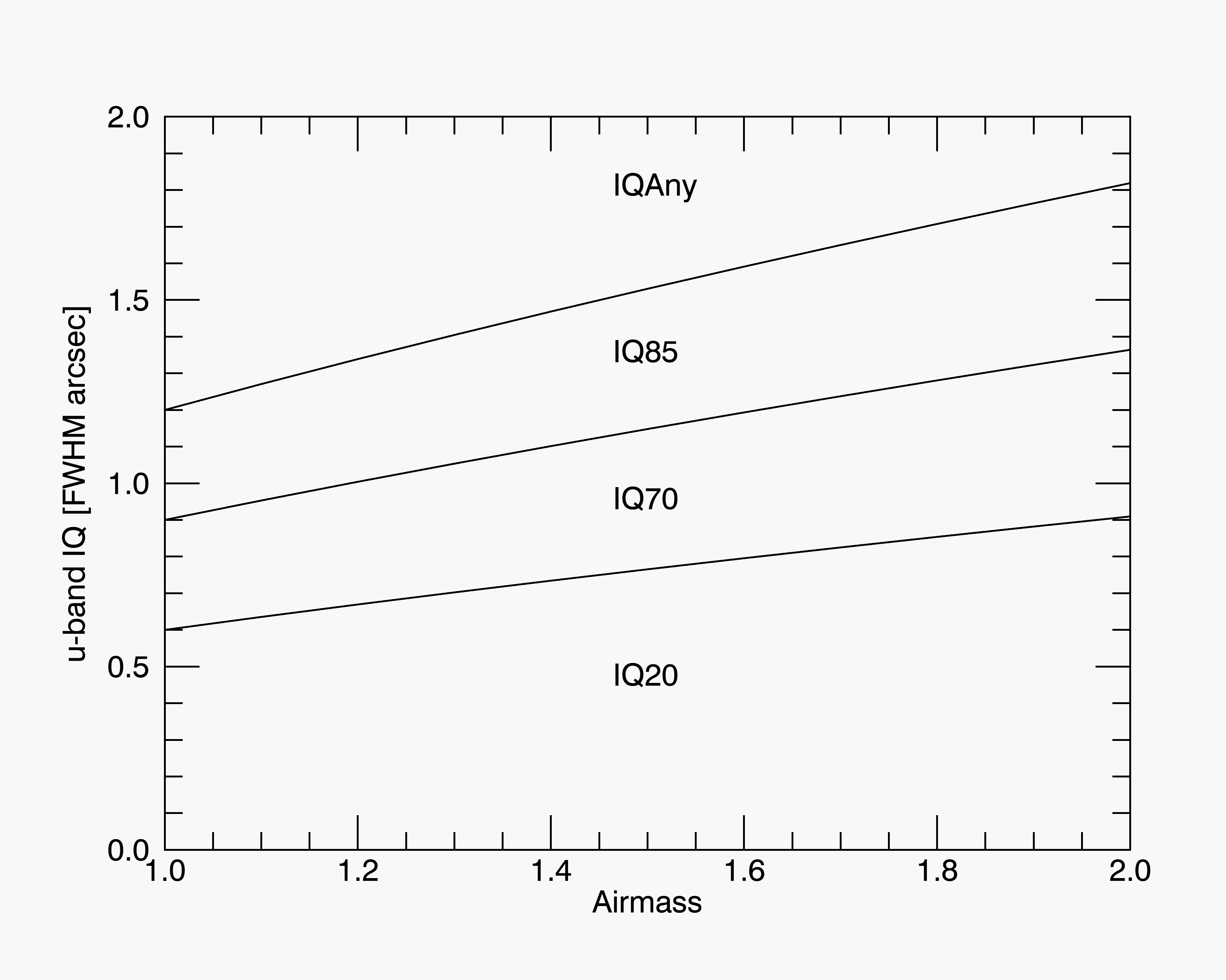
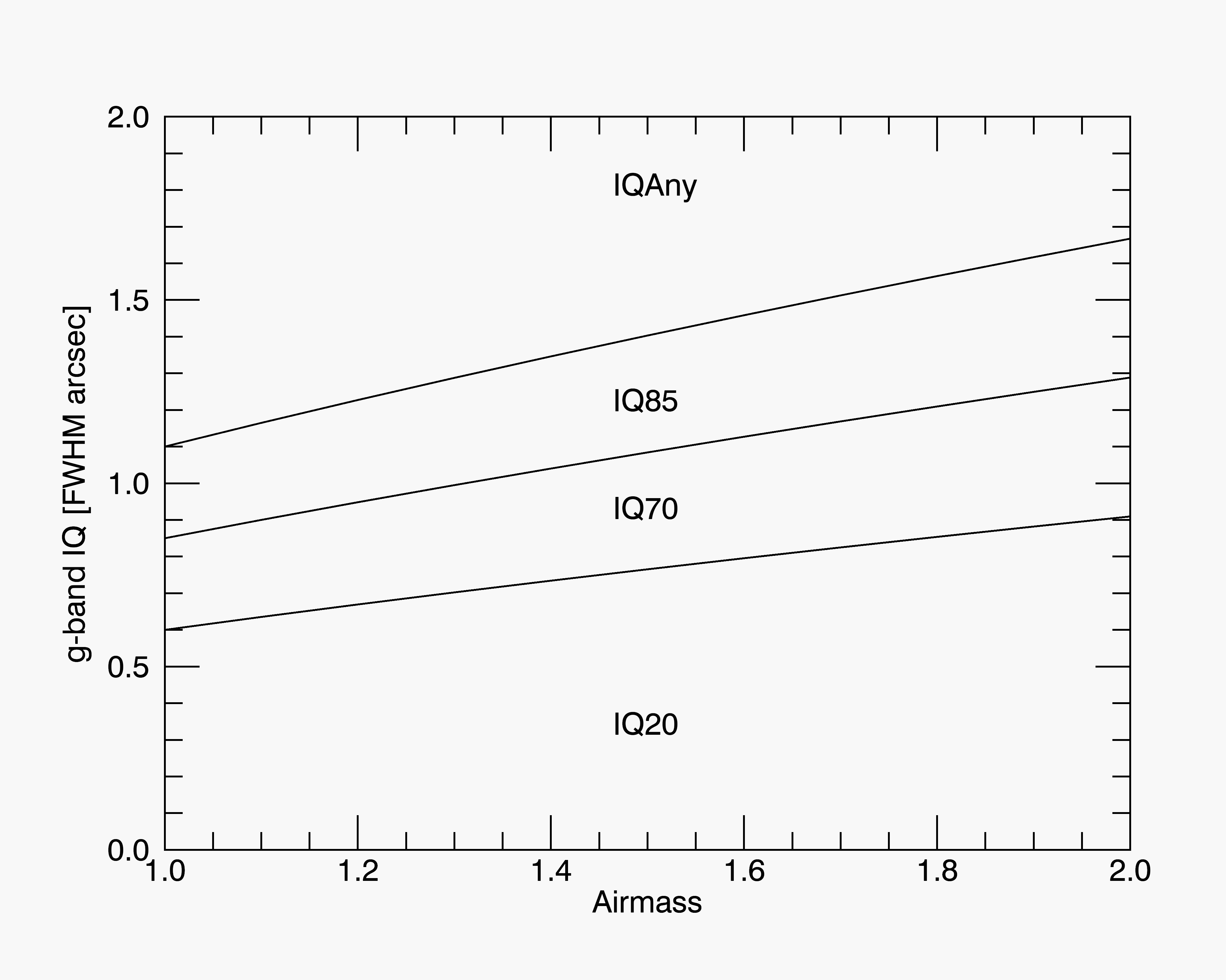
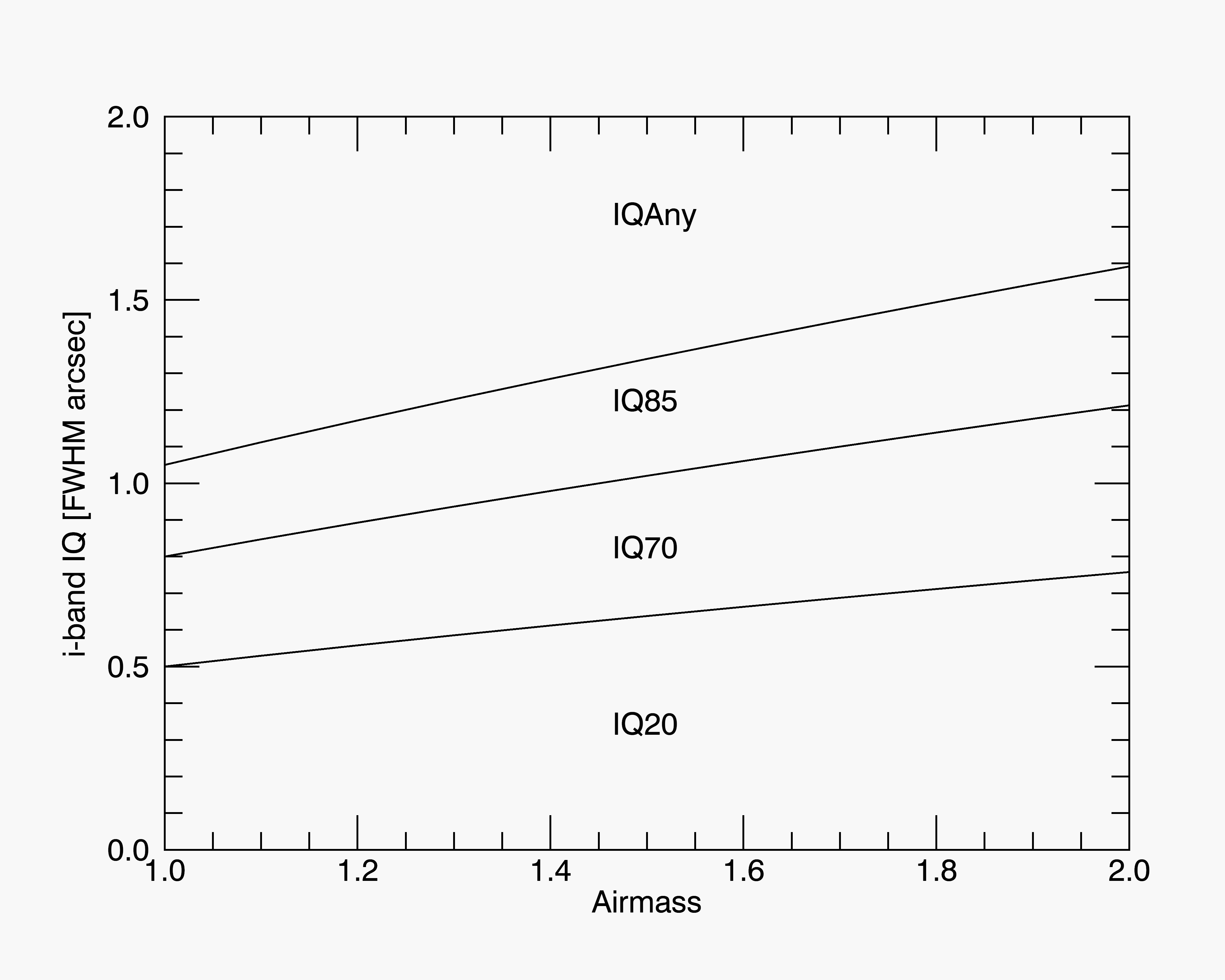
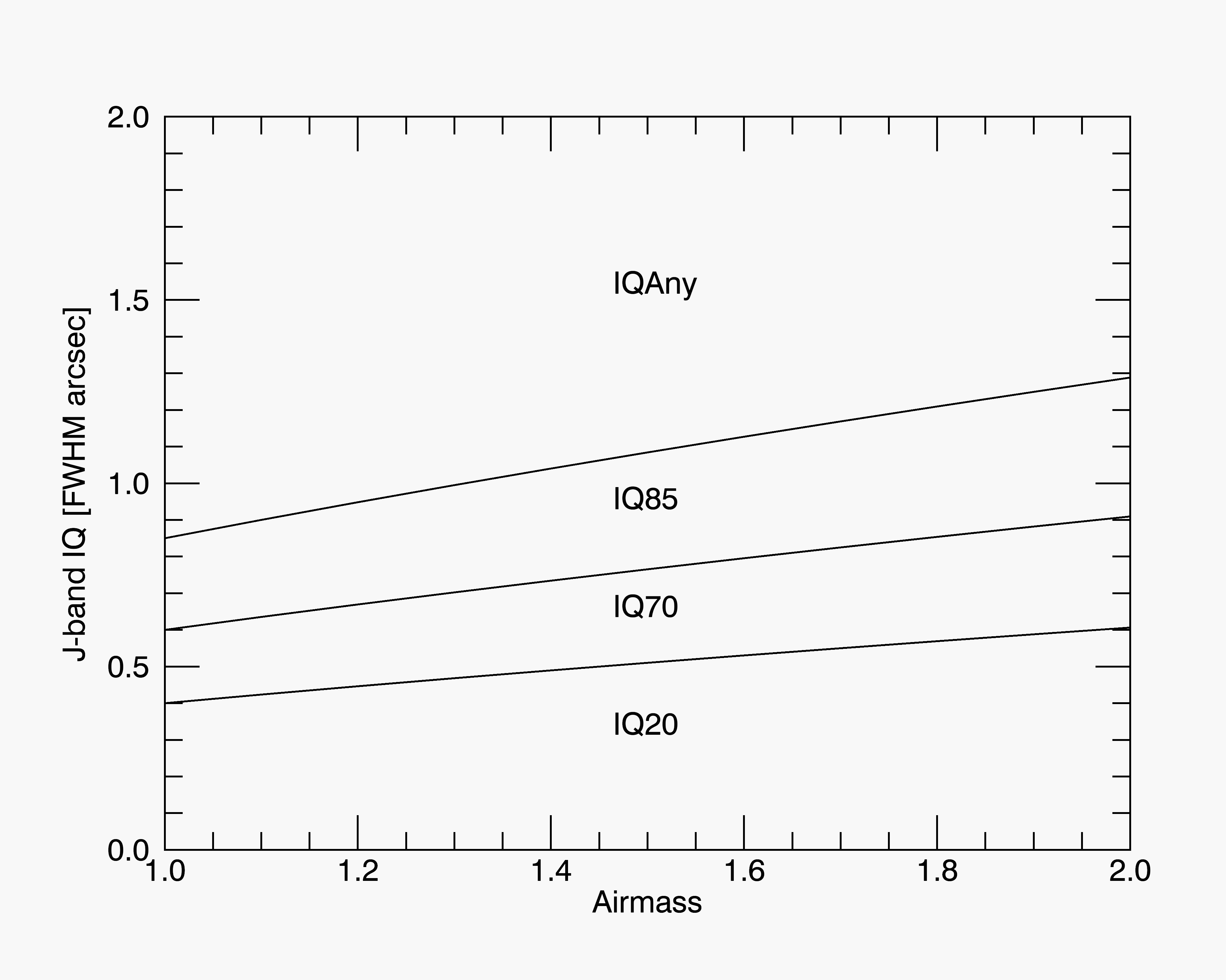
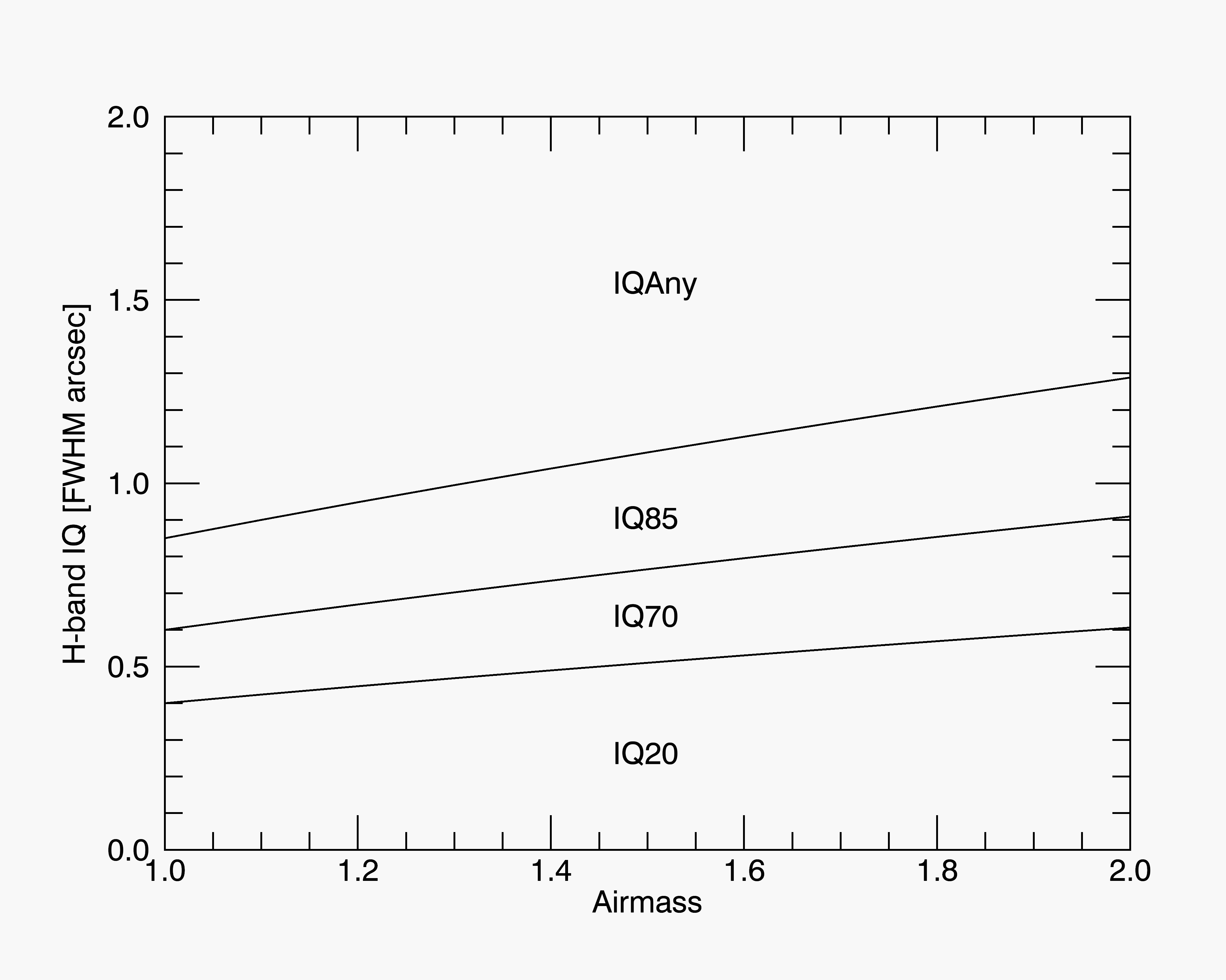
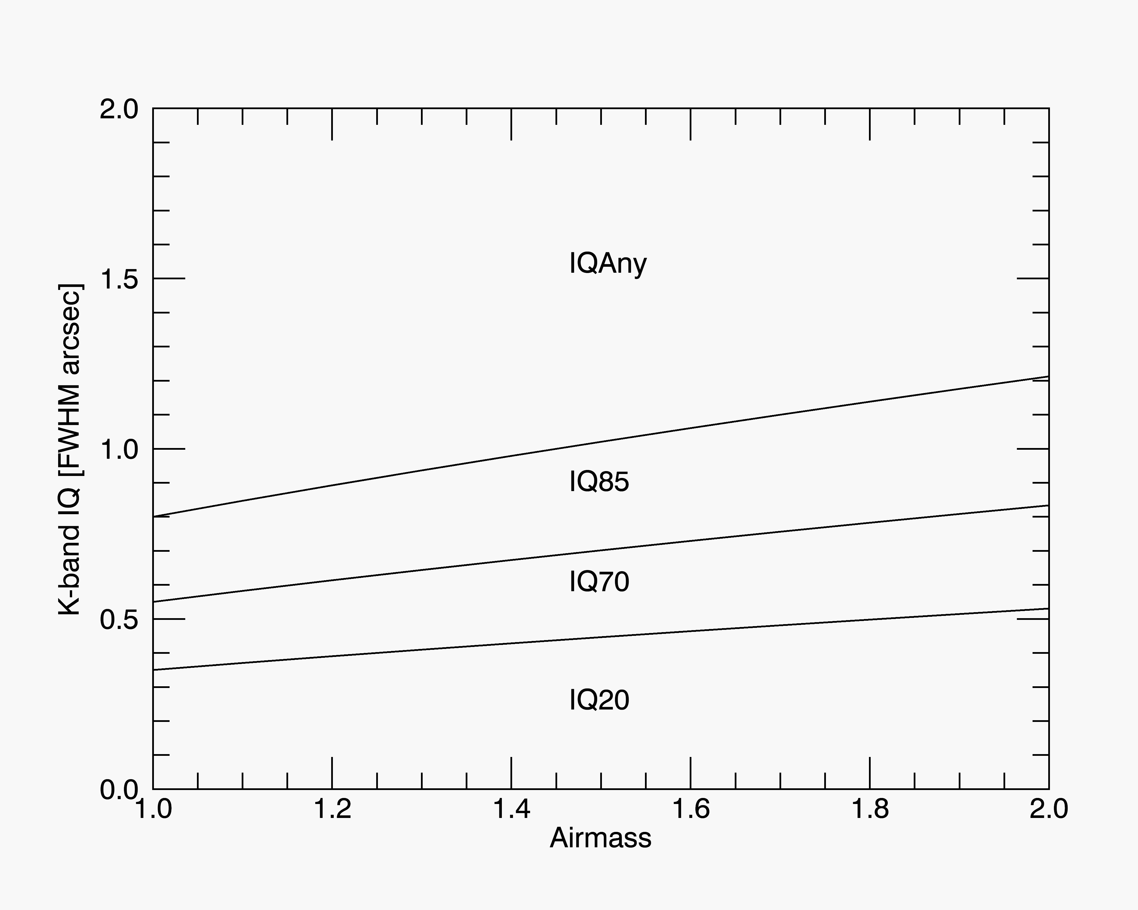
Delivered IQ Versus Airmass
The plots below indicate how delivered optical IQ (50% encircled energy) changes as a function of airmass for different image quality bins assuming IQ(X)=IQ(zenith)*X0.6. The delivered IQ for a bin is the region below the line above the bin label. The bin limits at zenith (airmass of 1.0) assuming use of the peripheral wavefront sensors are given on the Observing Conditions Constraints page.
u band (0.350 um)
g band (0.475 um)

i band (0.780 um)
J band (1.2 um)
H band (1.65 um)
K band (2.2 um)
Maunakea Water Vapour Statistics
Data logged continuously by the 225GHz receiver at the Caltech Submillimeter Observatory (CSO) over the periods 1994-1995 and 1997-1998 have been analysed. This equipment measures the zenith optical depth in the wing of an atmospheric water vapour line and may be used to derive the precipitable H2O column density above the site (Holland, W. 1999, personal communication):
mm of H2O = 20 * tau(225GHz)
A cumulative frequency histogram of the optical depth was generated for each quarter in 1994 and 1995:
![[cum freq histogram]](/sciops/ObsProcess/obsConstraints/csotau.gif)
and compared with data for 1997 to mid-1998 data available at CSO.
The following table shows the average optical depths and the values adopted for the Gemini observing condition constraints:
| Period | CSO 225GHz tau | ||
| 20%-ile | 50%-ile | 80%-ile | |
| 1994-1995 | 0.047 | 0.078 | 0.130 |
| 1997Q1 | 0.048 | 0.085 | 0.150 |
| 1997Q2 | 0.052 | 0.092 | 0.160 |
| 1997Q3 | 0.068 | 0.100 | 0.160 |
| 1997Q4 | 0.041 | 0.063 | 0.120 |
| 1998Q1 | 0.037 | 0.047 | 0.072 |
| 1998Q2 | 0.042 | 0.078 | 0.143 |
| adopted | 0.05 | 0.08 | 0.15 |
Thanks are due to Remo Tilanus for extracting the 1994-1995 data from the JCMT archive.