- PIO
- Sciops
- Gemini Home
- Telescopes and Sites
- Science Visitors at Gemini
- Observing With Gemini
- Instruments
- NORTH
- ALTAIR
- GMOS
- GNIRS
- NIFS
- NIRI
- SOUTH
- FLAMINGOS-2
- GeMS
- GMOS
- GPI
- GSAOI
- NICI
- VISITING
- Visiting Instrument Policy
- DSSI Speckle Camera (North)
- TEXES (North)
- RESOURCES
- Integration Time Calculators
- Adaptive Optics
- GCAL
- Magnitudes and Fluxes
- Near-IR Resources
- Mid-IR Resources
- Observing Condition Constraints
- Performance Monitoring
- SV/Demo Science
- Future Instrumentation
- Queue and Schedules
- Data and Results
- Helpdesk
- Statistics
Change page style:
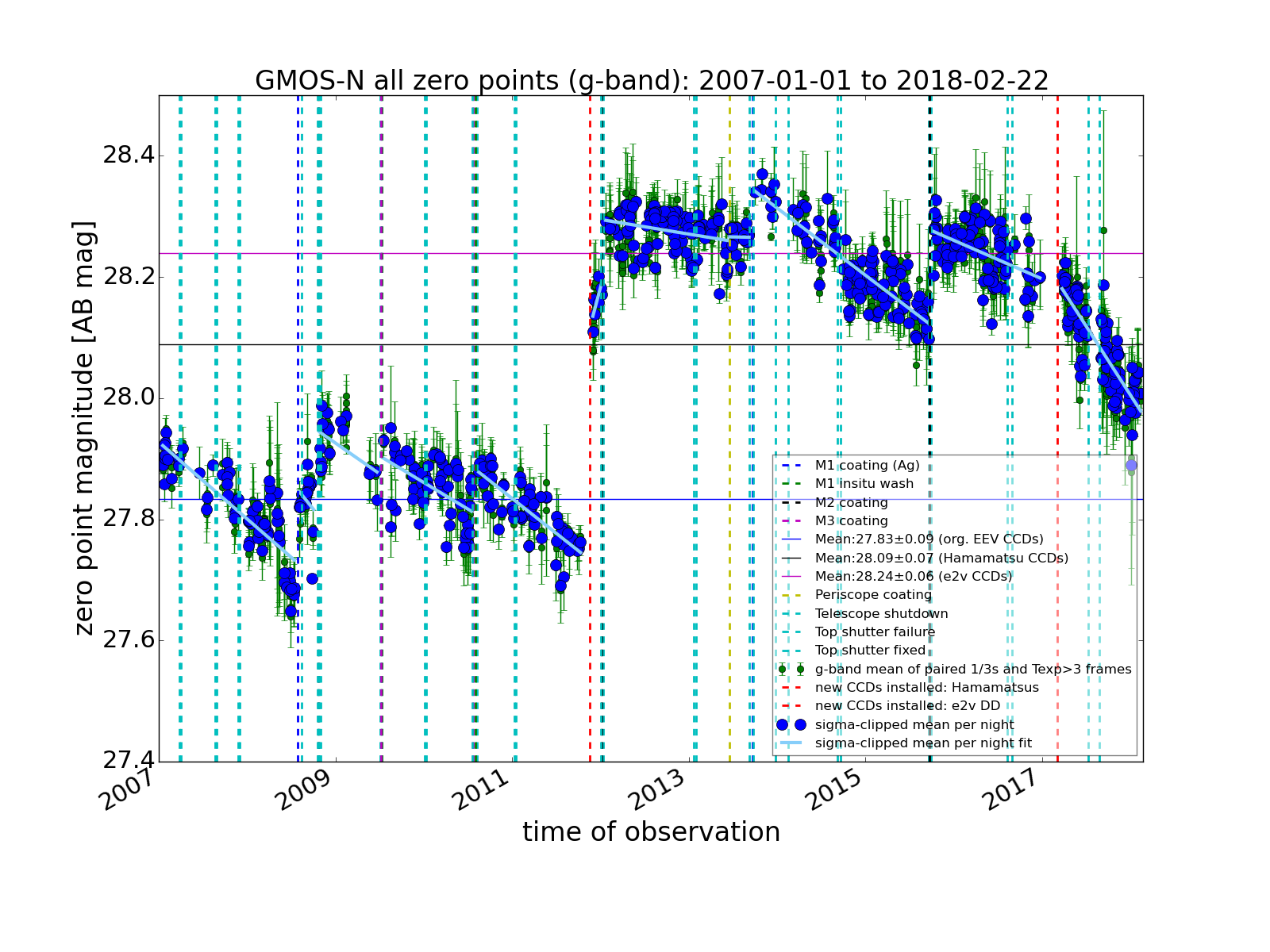
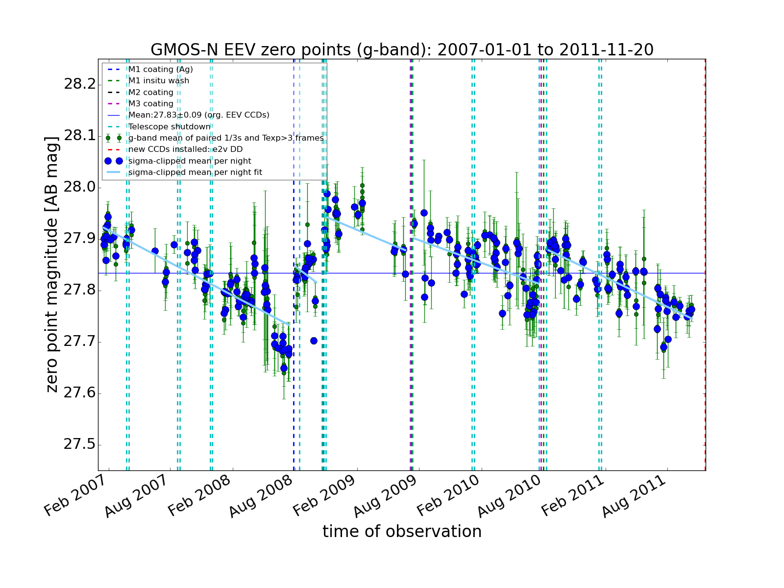
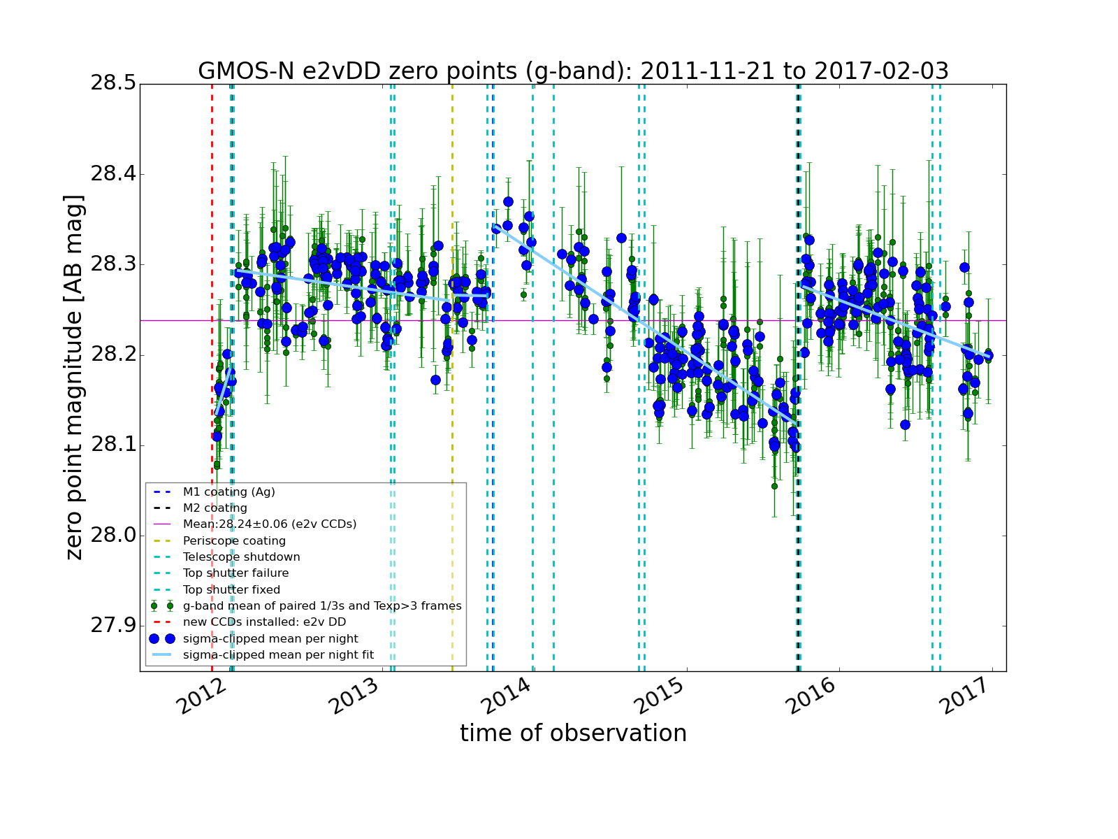
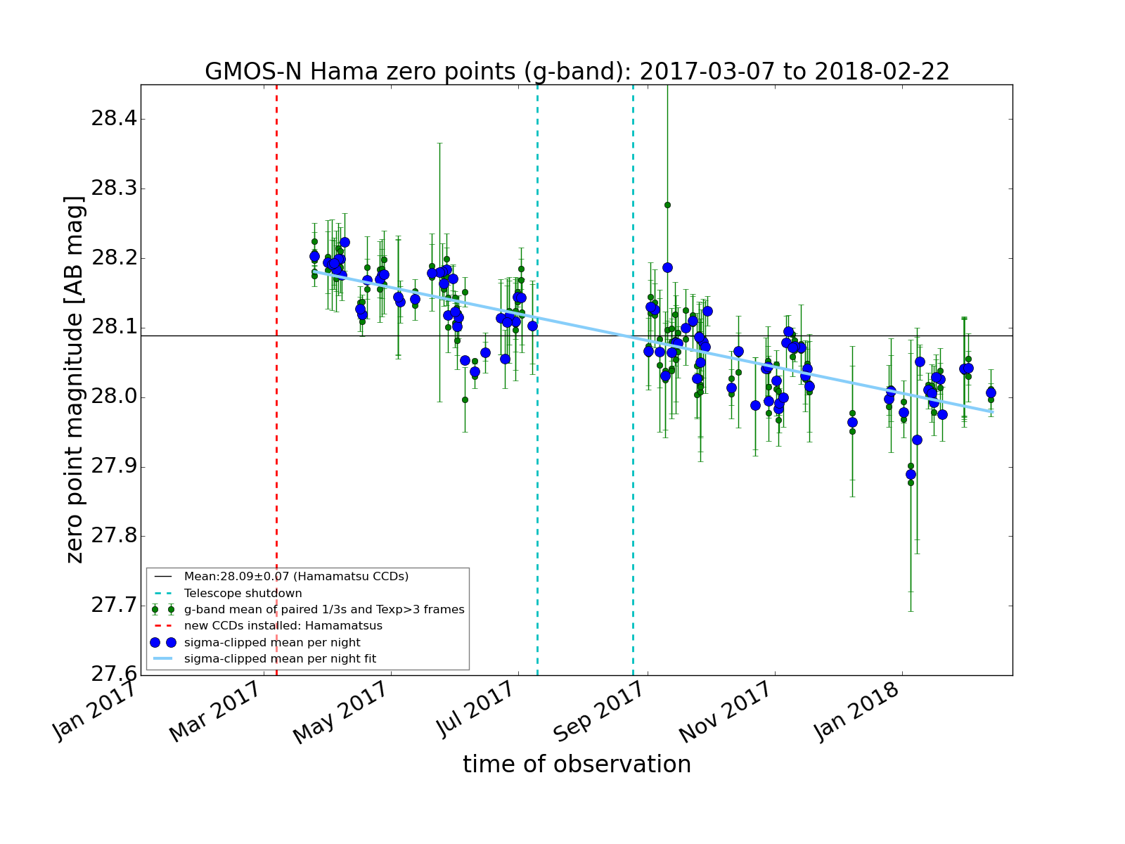
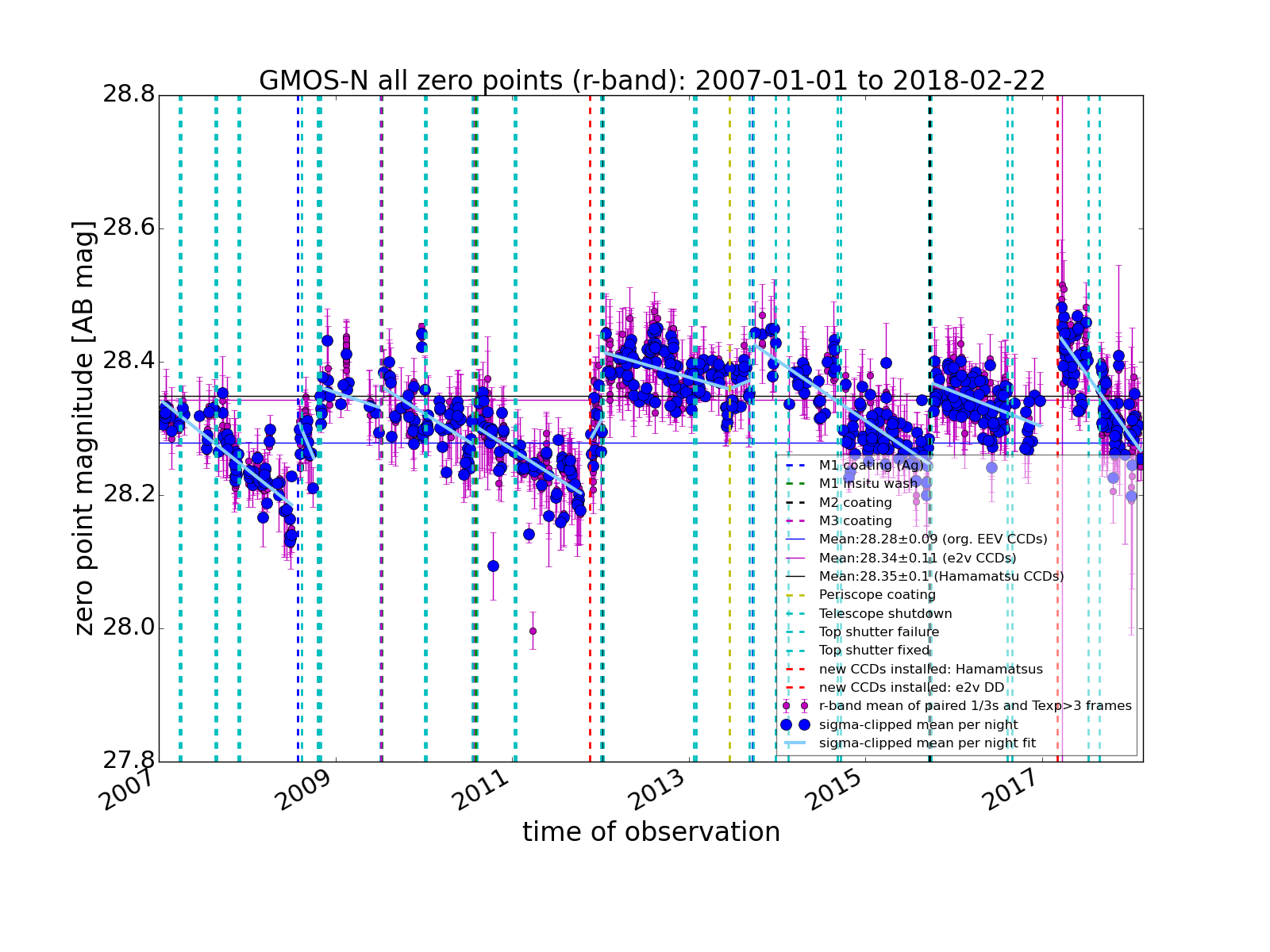
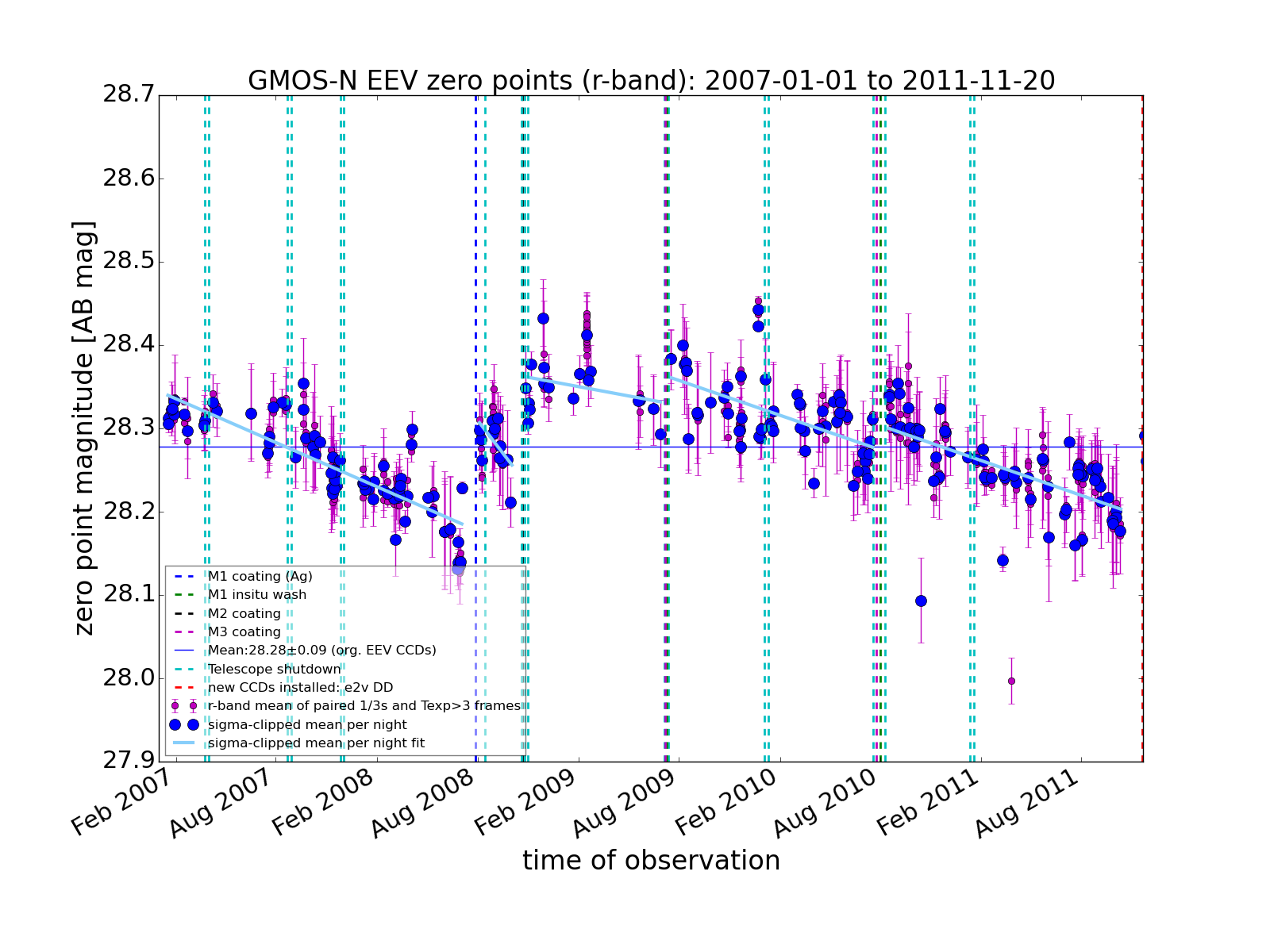
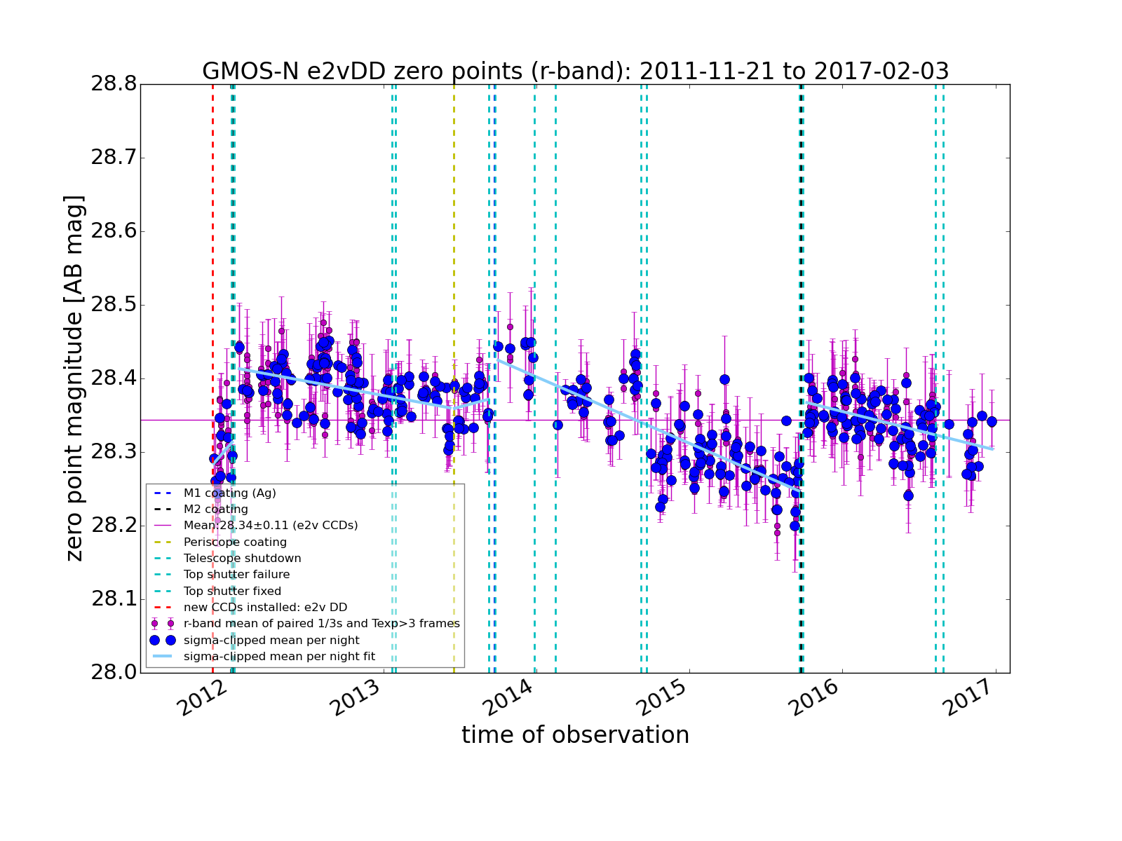
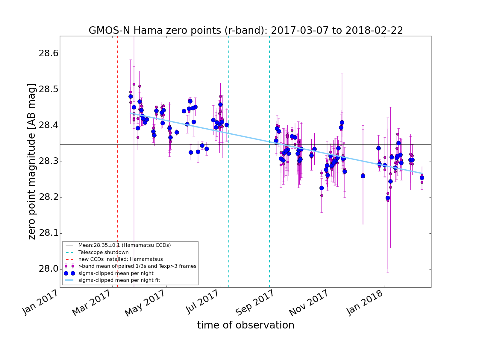
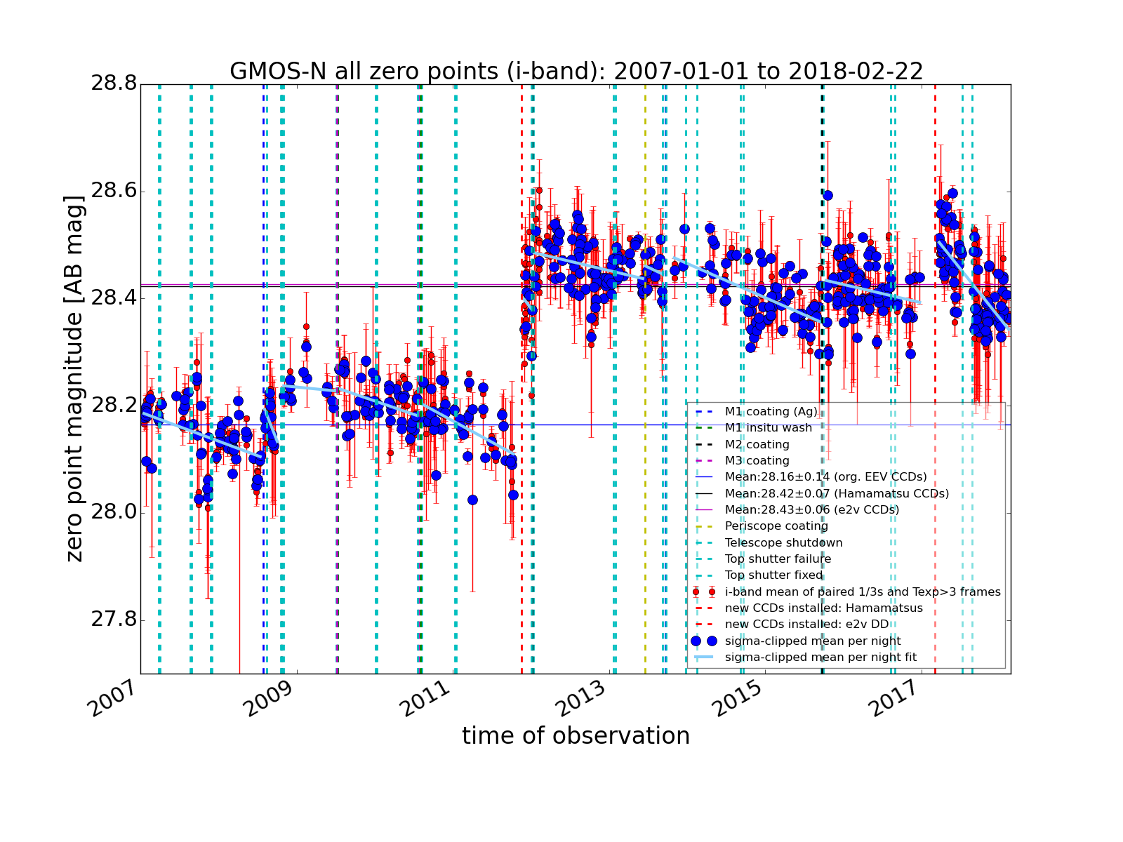
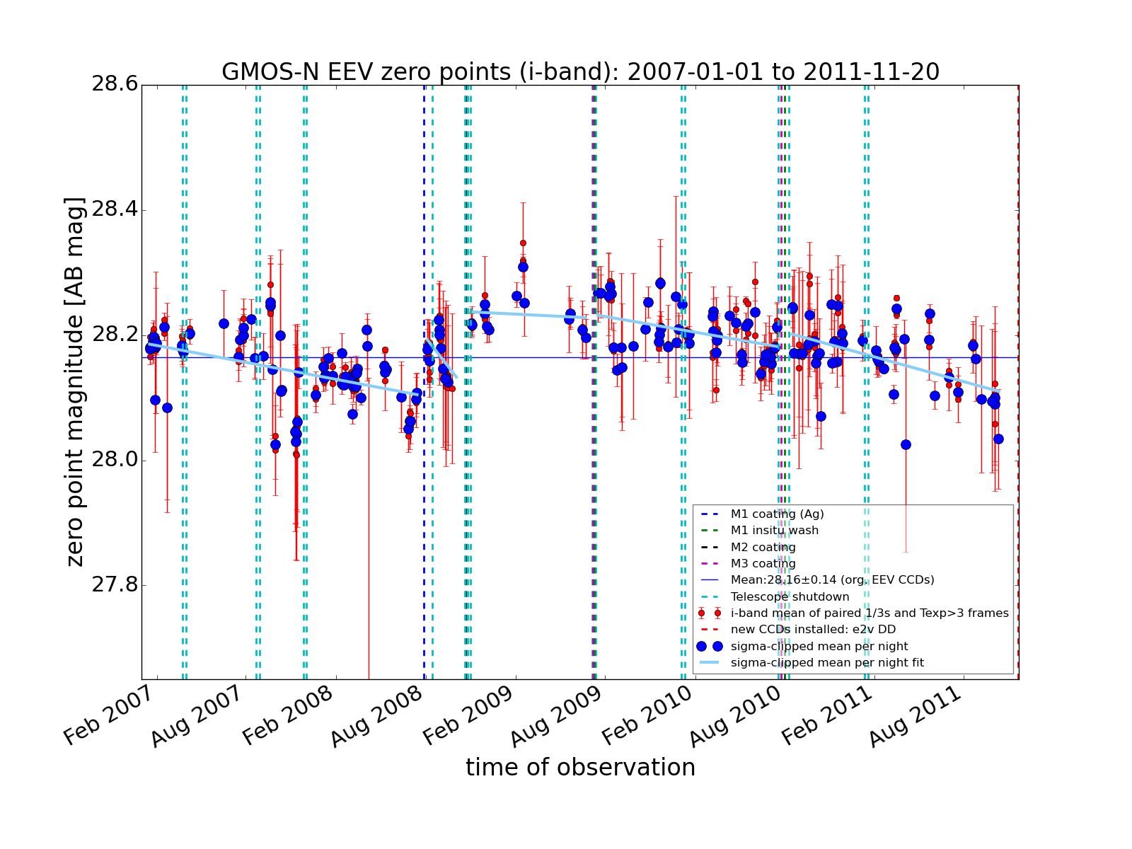
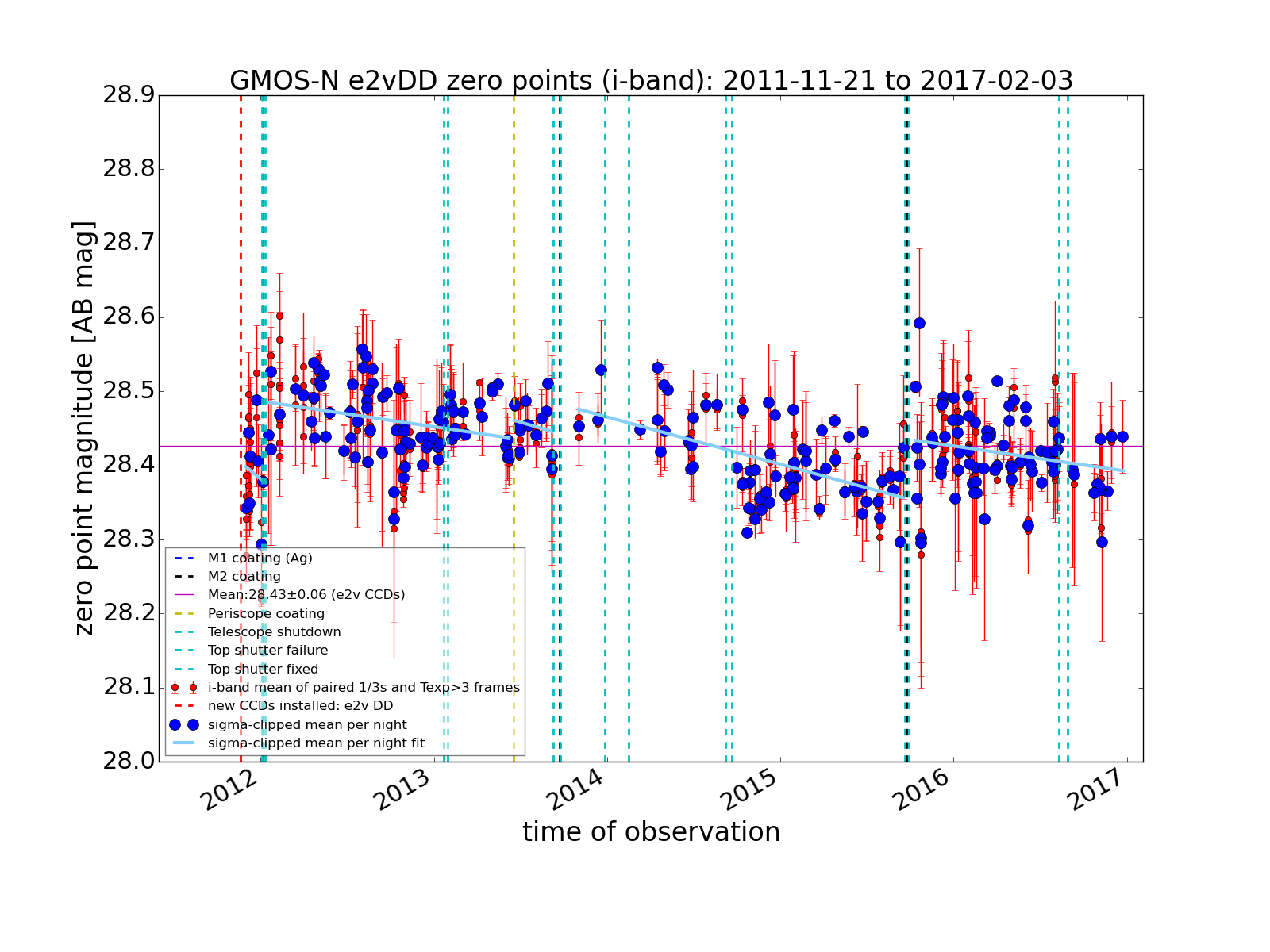
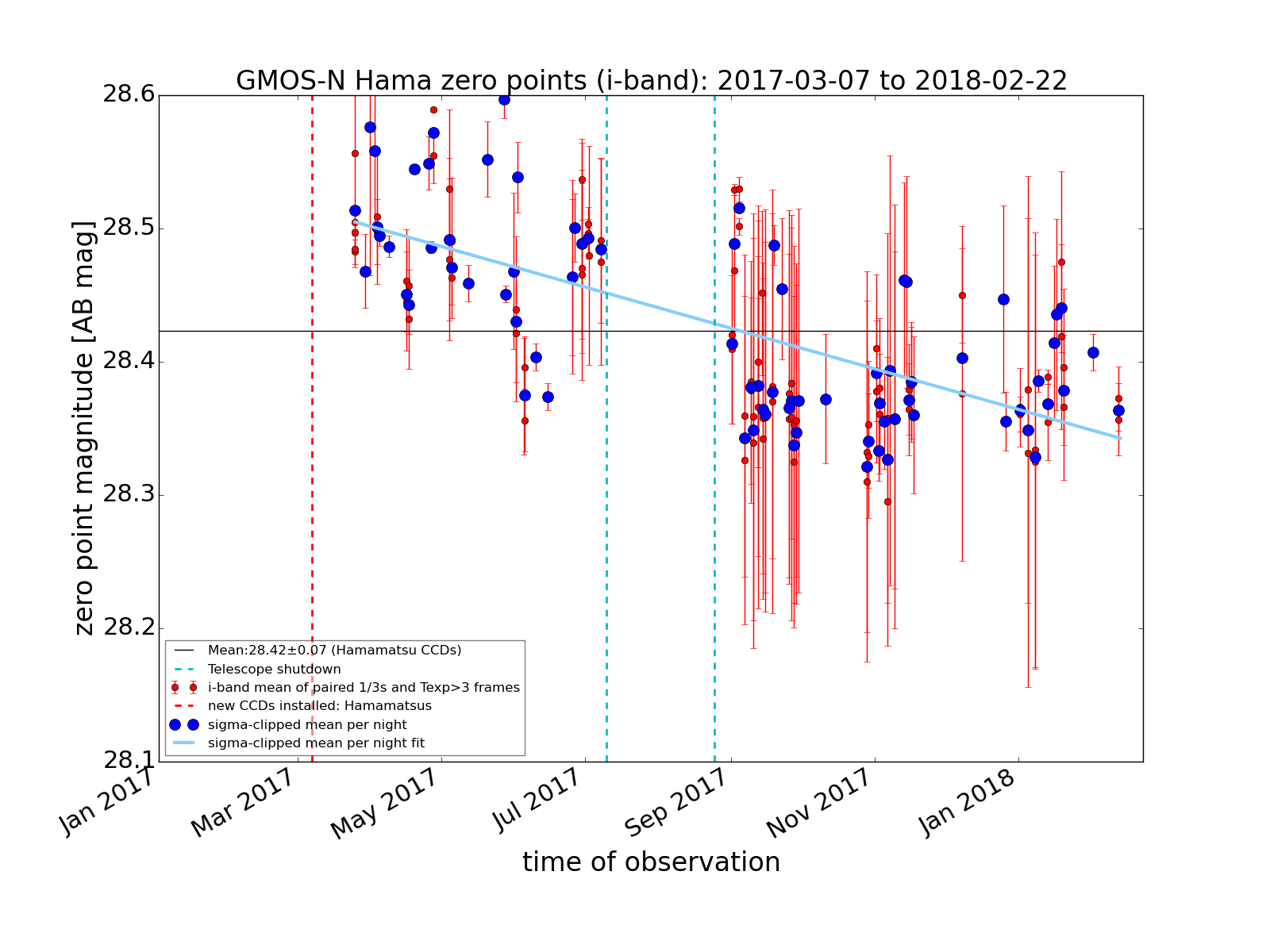
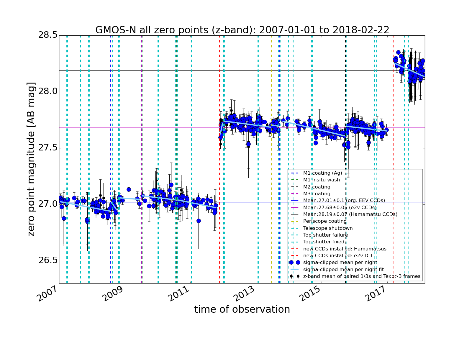
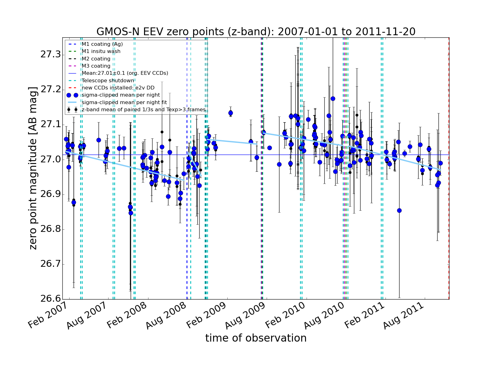
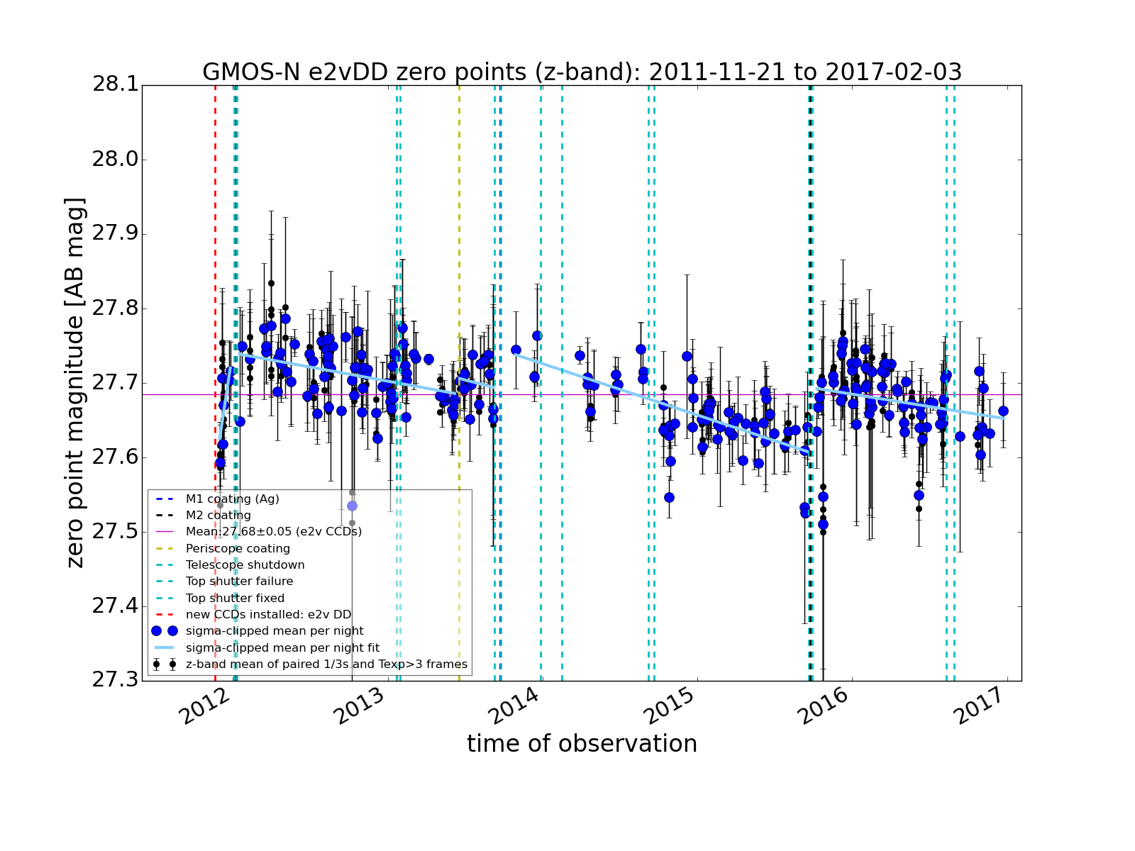
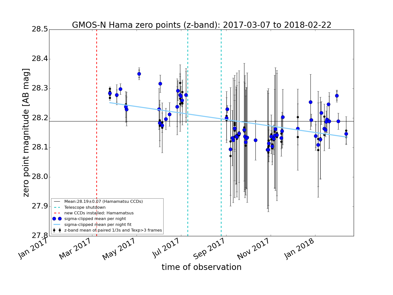
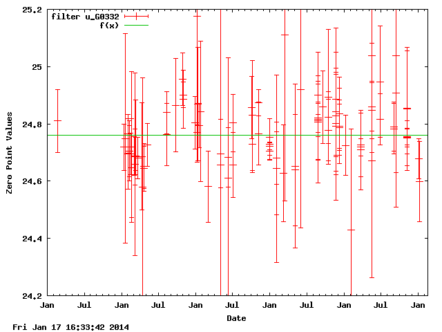
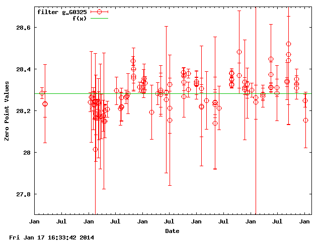
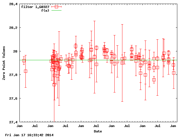
Photometric zeropoints
Imaging throughput is monitored in the form of photometric zero points for griz bands for GMOS-N, and ugriz for GMOS-S.
All photometric zeropoint measurements are based on observations of the photometric standards fields used by Gemini.
Usually the staff observer only obtained standard star observations if the night was judged to be photometric based on the counts from the guide-probes on Gemini and/or in the North the information from the Canada–France–Hawaii Telescope (CFHT) SkyProbe or the Mauna Kea All Sky Infrared and Visible Sky Monitor (ASIVA) run by the CFHT.
The AB zero-point magnitudes are given by:
mstd = mzero - 2.5 log (Ne/t) - k (AM-1),
where Ne is the background-subtracted number of electrons within the aperture, t is the exposure time, and AM is the airmass. The AB magnitudes were measured within an aperture that is equal to 4 times the FWHM of the images, so they are insensitive to seeing variations.
For GMOS-N the files and plots below contain all data taken since the start of 2007 run through an updated instrument monitoring pipeline which was introduced end of 2016 to replace the one running at that time developed in 2007 (see below for more details). For GMOS-S data from 2009 to 2014 is shown run with the old pipeline.
All standard star observations per night are averaged to give a nightly averaged zero point (ZP measured mean) tabulated in the datafile linked below. To account for the uncertainty caused by the GMOS blade shutter (i.e. the travel time for the shutter blades depends slightly on the direction of movement) all short integration time observation (Texp < 3sec) are taken in pairs of which only the average is used.
Large variations in the zero points are seen over periods of weeks to months depending on the state of the optical components, where M1 and M2 have the main effect. So we decided to derive a zeropoint per night based on the fit of all 3-sigma clipped, nightly averages between optical events (e.g. mirror coating or cleaning), thus being able to exclude skewed nightly averages e.g. by data taken in non-photometric conditions. This fitted zeropoint (ZP fitted) is also given in the datafile below as well as being marked on the plots together with the labelled event boundaries.
The quoted standard deviation of the measured values (ZP measured stddev) is the spread of the measured ZPs for all standard star pairs or stars with longer Texp observed within a night. For the fitted ZPs we use the spread of the offsets of the nightly average from the fit as the standard deviation (ZP fitted stddev). This value is constant over the range of the fit. For more details on the pipeline please see below.
| GMOS-S data analysed with older version of pipeline. | Site |
Band | Nightly averages |
Plot all CCDs |
Plot EEV CCDs |
Plot e2vDD CCDs |
Plot Hamamatsu CCDs |
North | g | datafile | Click | Click | Click | Click | North | r | datafile | Click | Click | Click | Click | North | i | datafile | Click | Click | Click | Click | North | z | datafile | Click | Click | Click | Click | South | u | datafile | Click | South | g | datafile | Click | South | r | datafile | Click | South | i | datafile | Click |
The instrument monitoring zeropoint pipeline for GMOS, a set of Python scripts, is running each day and looks for observation of fields from the set of standard fields used by Gemini (18 at GN, xx at GS).
If files are found the data is reduced using the GMOS specific Pyraf tasks provided by Gemini (gprepare, gireduce, gmosaic).
The pipeline does not use the overscan, but applies the best fitting (closest in time) biases and flats produced in the weekly/monthly reduction session of the calibration images taken.
Since the images are taken without dithers the chip gaps and CCD boundaries are filled with a mask value to be able to identify it later during the photometry.
In a first run we use IRAF's apphot phot task to identify the stars based on their catalogue position and the WCS of the images. Since the images are taken without acquisition, i.e. without pointing correction, and unguided this process isn't highly reliable. Mis-identifications do happen, but are almost always filtered by the pipeline in subsequent steps.
As a first check all offsets of the identified stars from their initial position are calculated. If the offset is exactly zero the star is excluded as the pointing is never perfect.
The remaining offsets are iteratively compared to the median offset removing the star with the largest offset if its larger than 30 pixels.
If only one star is left after this process for fields with more than two stars the images is excluded, as they are probably all mis-identified.
On the remaining stars an imexam 'm' is run to check for saturated stars. The pipeline defines saturated as being above a hardcoded, conservative non-linearity limit of 55k in ADUs.
Another imexam 'a' is then run on all the unsaturated stars to get an estimate of the FWHM, which is later used to determine the aperture size as four times the median FWHM.
Before averaging the measured FWHM to a single value per frame another round of excluding mis-identifications is performed.
For each successful detection the peak of the fitted imexam profile needs to be 1000 ADUs above the sky, and the allowed recentering in imexam should have been below 10 pixels compared to the original center estimated by the phot task. The whole frame is rejected if the mean FWHM is outside the reasonable range of 0.32 to 3.64 arcsec.
Another final sanity check is done now, by excluding images where only one star is left for fields with more than two stars, as they are probably all mis-identified.
For the remaining stars the sky background is determined as a sky per pixel using IRAF's apphot fitsky task. The sky annulus is set to the aperture plus a safety distance of 20 pixels and the sky dannulus is set to 10 pixels.
The final aperture photometry run on the stars is done using the Python photutils aperture_photometry task, which is more flexible in taking care of masked pixels compared to the tasks available in IRAF.
Using the X and Y centers obtained in the last imexam run aperture_photometry determines the total sum within a circular aperture, which is constant for each image.
To avoid getting skewed fluxes by stars close to the CCD gaps and boundaries a mask image is used in the aperture_photometry task, where all pixels with the above set mask value are excluded.
The final flux is the calculated as the total sum minus the corrected sky contribution, which is the area of the aperture minus the masked pixels within, times the value of the sky per pixel determined above.
The photometric error of the flux is calculated in the standard form as a Poisson noise based on the flux itself, the stddev of the sky value, the area, and the number of sky pixels. However, it turns out that this error is significantly smaller compared to the variations we see between zeropoints from different standard stars on the same field, so we don't use these in the subsequent analysis. The measured larger errors are from systematics not yet included such as colour terms.
Before writing the results of the aperture fit into the final photometry file, used to derive the nightly averages we quote in the datafile above, stars with negative flux, as well as star too close to the CCD gaps or the boundary are removed. Furthermore a hardcoded set of a few standard stars are removed due to various reason (e.g. having a close neighbour or being excluded by Jorgensen (2009) based on the colour-colour diagram of an older subsample of GMOS photometric standard observations which they analysed).
Please note, the new 2016 pipeline does not significantly change the derived zero points compared to the old 2007 pipeline, e.g. the mean value for the e2v DD CCDs is now only 0.01 to 0.02 mag larger for all bands. What has significantly changed is the spread in the measurements, e.g. the g-band stddev went down from 0.22 to 0.06 mag. This brings out now with more clarity the expected systematic degradation of the mirror between re-coatings. The main improvements responsible for this are coming from a more careful treatment of mis-identifications or unreasonable measurements throughtout the pipeline run and an improved treatment of masking the gaps and borders.