Announcements
Learning the OT tool
In Phase II, is when you have to define concisely your observations; Phase II submissions are required to contain spectroscopic acquisition sequences and all calibrations. These observations are automatically generated by the Observing Tool (OT), although they will need customising for the PI's particular use case (e.g. adding telluric standard star coordinates).
The GNIRS team strongly recommends that users start from the automatically-generated OT templates and the GNIRS OT library when preparing GNIRS observations. The library contains detailed instructions for customising the template observations: changing targets, standard stars, slit widths, wavelengths, etc
In this section a generous information is provided with the aim that you will be able to use efficiently this software in order to define the observations of your program. The best way to approach to OT is to watch the suite of dedicated tutorial videos. Below, you can find a more detailed description of how to use OT for your GNIRS observations. However, if you still are still hungry for more information about Phase II in general, please don't hesitate to visit this webpage.
GNIRS in the Observing Tool
This section is intended to explain the various OT components in more depth:
As well as the science target spectroscopy, GNIRS programs must include:
- Acquisition observations for all targets
- Calibration observations: telluric standards, flatfields and arcs; any additional calibrations
After creating your GNIRS observations, please check the Checklist. If you still have questions, submit a HelpDesk query.
The GNIRS Static Component
Adding a GNIRS component to an existing observation, or adding a "GNIRS Observation" gives access to the GNIRS static component. The GNIRS component is used to define the basic GNIRS configuration and looks like this:
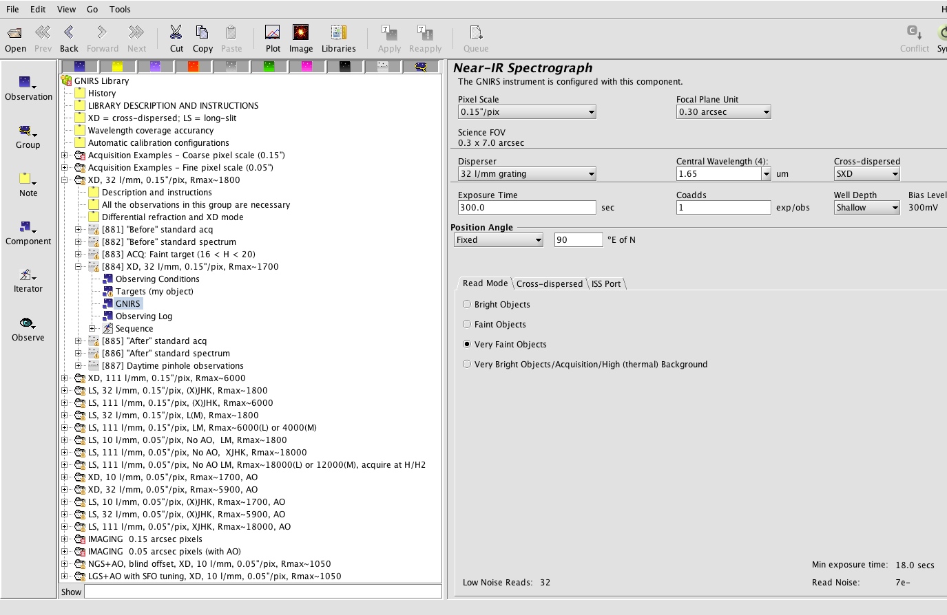
The available items are:
- The combination of pixel scale and central wavelength (below) determines which of GNIRS' four cameras is selected. 0.15"/pixel selects one of the "short" cameras, and 0.05"/pixel selects a "long" camera. The science field of view (shown in green) will update to reflect the configuration chosen, also displayed by the position editor.
- The disperser menu is used to select one of the three gratings. This, in combination with the pixel scale and slit width, determines the spectral resolution.
- The minimum exposure time is 0.2 sec, maximum exposure is generally dictated by object brightness, sky background or radiation events (see the Observing Strategies and Known Issues pages). Coadds can be used to combine multiple integrations, useful for high background observations or other situations in which exposures are very short.
- The focal plane unit menu is used to select the slit width or the IFU mode. The slit length is determined by a separate mechanism (the decker) which is implicitly determined based on the pixel scale and whether one of the cross-dispersing prisms is used.
-
The central wavelength field sets the grating central wavelength. Menu choices are available and recommended for moderate dispersion (0.15"/pix + 32 l/mm grating) configurations. For higher-resolution observations, any wavelength can be entered. The proper order-sorting filter is automatically selected; this choice can be overridden using the GNIRS iterator, although this is normally only necessary for acquisition observations.
- The cross-dispersed menu selects whether a cross-dispering prism is used for the observations and if so, which one. For short-camera cross-dispersed observations, only one XD prism is available. With the long camera, either the SXD or LXD prism can be chosen. This choice has implications for slit length, wavelength coverage and spectral resolution.
- Well Depth: the bias voltage may be adjusted to increase the well depth for thermal IR (L and M band) observations or observations of very bright targets. The default is "shallow", which is appropriate for most observations below 2.5 microns.
- Position angle: this may be set to "Fixed" or to "Average parallactic." In the latter case the value for the PA will be selected at the time of observation. Selecting the average parallactic angle minimizes slit losses, but is only important in cross dispersed mode with the narrowest slits. See the refraction table for more information. If a fixed angle is selected a value of 90 degrees is recommended; it usually minimizes drift perpendicular to slit due to flexure between GNIRS and the peripheral wavefront sensors. However, any position angle - specified in degrees E of N - may be chosen. The view of the science field in the position editor will reflect the selected angle.
The read mode is automatically set when defining the exposure time for the integration, although the user can override this choice. Each read mode has a different read noise and readout overhead: see the detector and observing strategy pages for more details. Green text is informational.
The ISS port tab allows the user to select the position on the Instrument Support Structure in which GNIRS will be used. Changing the choice of port selection alters the way the field of view is displayed in the position editor, as well as various configuration options set at the telescope. GNIRS is going to be mounted on the side port from 2011A for the foreseeable future, so "side-looking" (the default) should be chosen.
To make any changes visible in the observing database used by the observatory, the program must be stored.
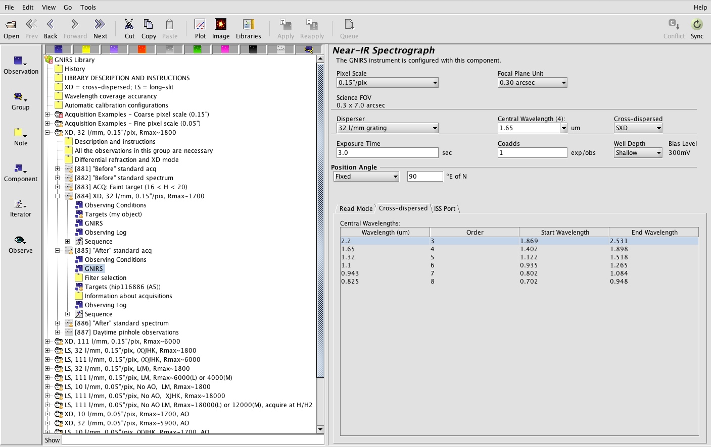
Selecting cross-dispersed (XD) mode
When a cross-dispersing prism is selected, the cross-dispersed tab becomes active (shown below). This tab displays the full wavelength coverage provided by orders 3 through 8, the primary orders passed by the cross-dispersing prism. This is an informational tab only, no input is required. With pixel scale = 0.15 arcsec/pix and the 32 l/mm disperser (max. R~1700), the central wavelength should be set to "cross-dispersed" (=1.65um). The observed spectrum will then provide essentially complete coverage from 0.9 to 2.5 um.
The GNIRS Iterator
The GNIRS Iterator is a member of a class of instrument iterators. Each works in basically the same way, except that different options are presented depending upon the instrument.
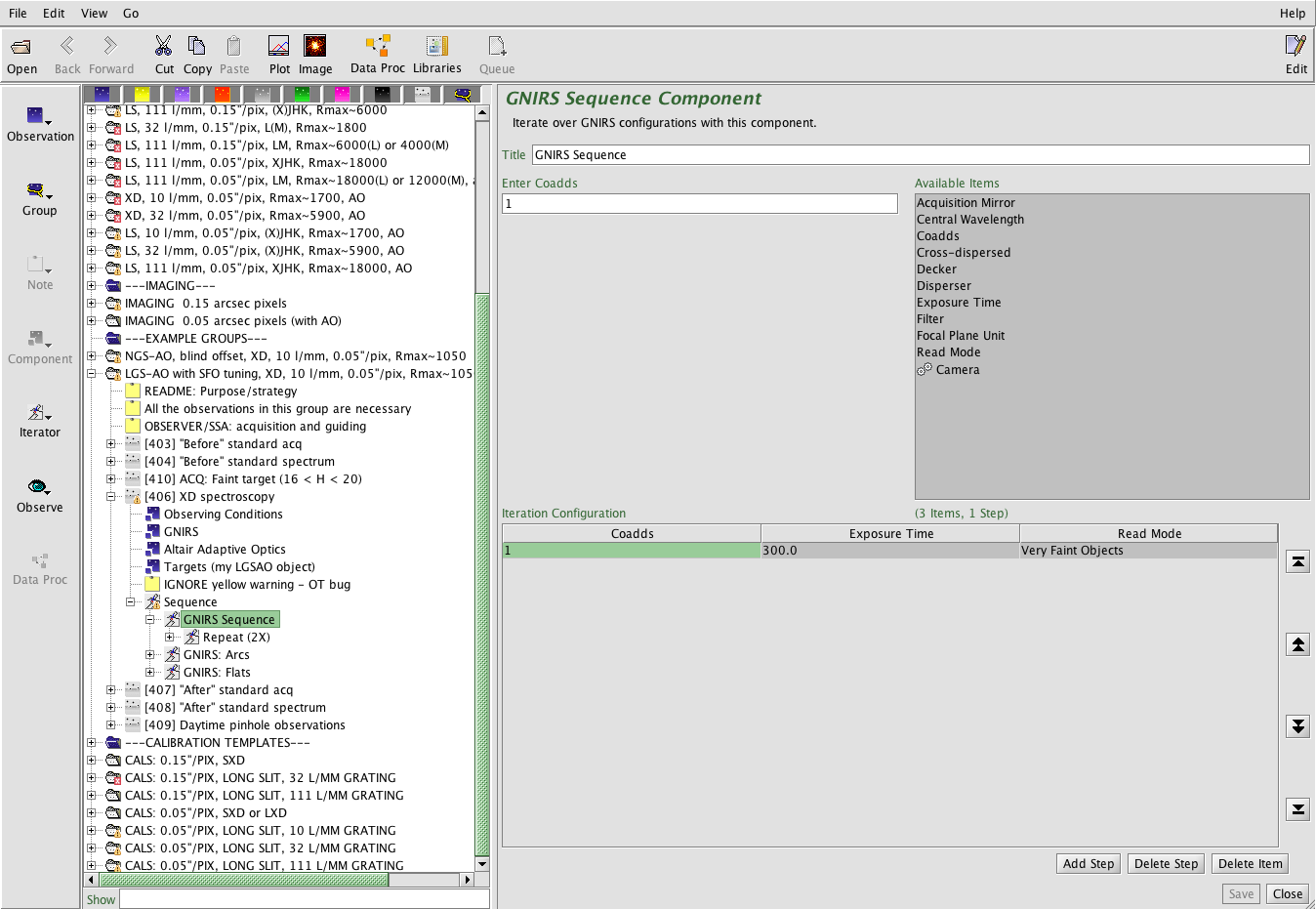
GNIRS iterators are required when the observation is stepping through different GNIRS configurations or - as is usual - flats and arcs are embedded in the observations (so that the appropriate read mode, which is not necessarily that used for the science exposures, can be selected for the calibrations). If you are iterating over GNIRS configurations and also dithering, the offset iterator would normally be nested inside the GNIRS iterator, and the observe command nested inside the offset iterator.
A good way to check your observing sequence is by clicking on the "Sequence" folder. There one can view the sequence as a contiguous list of actions or as a timeline.
The Offset Iterator
The offset iterator (visible in the above figure) is common to all instruments and is used to define the sequence of dithers or sky offsets to be used. The observing strategies page gives information on some of the considerations to be taken into account when setting up offset sequences for GNIRS. The offset sequence can be visualised using the position editor.
GNIRS in the Position Editor
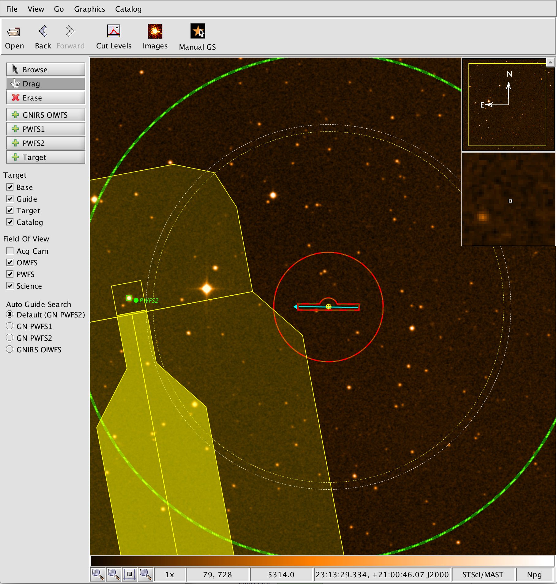
The position editor can be used to visualise the field of view and offset pattern, select and view guide stars, change the position angle, and much more. Full details of its capabilities are given on the generic position editor page. Here we point out that selecting the OIWFS causes the position editor to overlay a red, shaded "keyhole" corresponding to the science field of view in GNIRS' acquisition imaging mode (see figure below). This can be useful in planning acquisitions of complex fields, for example. The OIWFS itself has not been commissioned.
Acquisition Observations
Acquisition observations are needed for all on-sky observations (science targets and standard stars) and are defined in a separate observation from the spectroscopy observations. The OT library provides templates for acquiring several types of object:
- Very bright objects requiring use of a narrowband filter
- Objects faint enough to use a broadband filter, but bright enough that no sky subtraction is necessary
- Faint objects requiring sky subtraction
- Very faint objects requiring a blind offset from a reference star
The acquisition procedure is explained here.
The library notes give detailed instructions on how to customise the acquisition templates. In the static component, all fields except the exposure time, coadds and read mode should remain the same as in the spectroscopy observation. Although the grating is bypassed by the acquisition mirror, keeping the central wavelength and grating selection fixed avoids the grating being moved between acquisition imaging and spectroscopy (and thus between the science target and telluric standard). Near-IR acquisitions for thermal-IR observations should normally keep the deep well setting used for the spectroscopy, as the detector takes a few minutes to stabilise after changing the bias voltage.
In the GNIRS iterator contains the following steps, in which the acquisition mirror, coadds, decker (which determines the slit length), exposure time, filter and focal plane unit (slit) need to be set.
- Image of the slit. Slit image exposure times are typically just a few seconds (except in the narrowband H2 filter, which should not be used for slit imaging). The focal plane unit should be the same as that used for the spectroscopy, and the decker should be set explicitly and match the spectroscopy configuration. In the library templates the slit image is offset by 10" to avoid bright targets landing in the middle of the slit, making it difficult to measure the slit centre.
- Image(s) of the target field, with optional sky subtraction. The slit and decker should be set to "acquisition" for these steps, to allow the whole imaging field of view to be seen. The exposure time and coadds should be appropriate for the source being acquired (see this table).
- Image of the target through the slit. This step should use the decker and FPU of the first step, but the filter, exposure time and coadds of the second step.
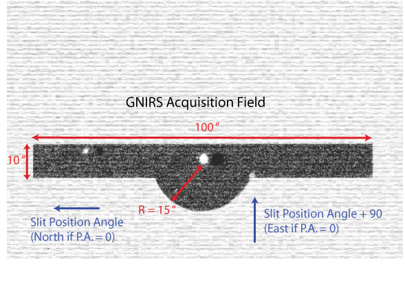
The acquisition mirror should be "in" for all acquisition observations. The GNIRS acquisition field scale and orientation are shown here, and can also be seen using the OT position editor as described above.
The red cameras, which are used for L/M band spectroscopy are sensitive enough at short wavelengths to be useful for H/K band acquisitions (see this page). This may be preferable to acquiring in the PAH band filter for some objects. The OT will give an error if the H band filter is selected for use with a red camera. This can be ignored and will be removed once software effort has been released from other tasks.
Acquisition time is charged according to the type of target, i.e., to the program for science targets, to the partner for baseline tellurics. This is accomplished by setting the Observe Class to "Acquisition" or "Acquisition Calibration", respectively.
Calibration Observations
PIs are asked to specify all calibrations, including baseline calibrations, in their Phase II OT file. The OT library example groups include telluric standards, flats, and arcs, and users are encouraged to take these groups as a starting point for defining their own observations.
Baseline calibrations generally consist of "before" and "after" telluric standards and GCAL flats, arcs and - for XD spectroscopy - pinhole flats. Calibrations in addition to the baseline set will be charged to the program, unless they can be executed between morning and evening twilight (e.g., darks, twilight flats). Flats and arcs that are taken with the data (i.e., without changing the instrument configuration) should be embedded inside the science or telluric observation. Using the "Night Baseline GCAL" option in the OT, as shown in the OT library examples, will automatically add the appropriate nighttime calibrations with the correct exposure times etc.
In principle it is possible to define single science observations containing several central wavelengths, taking arcs and flats at each wavelength before moving the grating to the next wavelength setting. However, such a sequence would involve moving the tertiary ("science fold") mirror between its sky --> instrument and GCAL --> instrument positions. The science fold mirror positioning is not reproducible enough to guarantee that the source will stay in the slit after a move, so we do not recommend this kind of observing setup (and this is one reason why the library examples all have the calibrations at the end of the sequence). PIs wishing to embed flats/arcs at multiple wavelengths should contact their NGO/contact scientist before proceeding.
Telluric standards should be defined in much the same way as a normal science observation, including an acquisition observation and the desired offset sequence. The only difference is the "Observe Class" which should be set to "Nighttime Partner Calibration" for baseline standards, or "Nighttime Program Calibration" for special/additional calibrations.
Observing Strategies
This page brings together information that might affect decisions on observing strategy in various GNIRS observing modes, and provide guidelines/tips to maximize observing efficiency and avoid some common errors. The other GNIRS web pages (and especially the Known Issues page) also give information about what to expect from the instrument. For information about actually setting up observations in the Observing Tool, please see the Observation Preparation section of these pages. If you discover errors or inconsistencies, please let us know!
Factors the PI may wish to take into account when designing observing sequences:
- Read modes, observing overheads and read noise
- Considerations affecting the maximum recommended exposure time
- Optimal design of the telescope offset sequence
- Slit orientation, taking into account the science needs, the importance of minimizing the likelihood that the target will drift out of the slit, and the importance of differential refraction
- The effect of slit width on signal-to-noise ratio in the J, H, and K bands where due to the plethora of narrow but strong OH sky lines, the noise varies rapidly with wavelength.
Read Modes
In the OT the read mode is automatically set based on the length of the individual exposures. However, its choice is not always the best one, because the OT does not take into account the background in the chosen wavelength range, or the brightness of the object to be observed. The choice of read mode can be edited to suit the user's needs. The following example illustrates the issues:
- The user wishes to observe a L=12.0 vega mag star from 3.35µm to 3.65µm at R~6000. She selects the 111 l/mm grating and the short camera, the deep well mode (180,000e) and an exposure time of 30 seconds. As soon as she enters 30 seconds the OT selects the faint object mode, which has a readout overhead of 9.0 seconds and a read noise of 12e according to the Detector properties webpage. A check of the GNIRS ITC shows that the signal from the star in the peak row is ~200e. The shot noise associated with that is 14e, so if that were the only criterion, the choice of read noise would be correct. However, the ITC plot also shows that the square root of the background is 100e or higher in this wavelength range. The background fluctuations thus dominate the noise and would do so even if the bright readmode (readnoise = 38e) were chosen. Since the bright read mode has an overhead of only 0.6 seconds, the user should select it in the OT.
Maximum Exposure Times
The maximum exposure time you should use is set by several constraints:
- Saturation on the sky
- Saturation on the object
- Sky variations during a dither sequence
The GNIRS exposure times page gives safe limits for currently available configurations. You can check background in the ITC for any configuration by squaring the background value shown in the result, and then dividing by the number of pixels in the software aperture used. The background per pixel should be kept at ~50,000 electrons maximum for shallow well (K and shorter wavelengths), and ~100,000 for deep well (L, M). We recommend individual exposures generally not exceed 900 seconds.
Bright objects may saturate the array before the background does. Check the recommended exposure times and scale the values to your particular case. You can check for object saturation with the ITC by selecting the star brightness and the instrument configuration and, in the "Analysis method" section, selecting "Software aperture of diameter" equal to the pixel scale (i.e., 0.15 or 0.05 arcsec); you will then see the spectrum in the peak row of the array only and will be able to judge if it saturates the array. If your program uses cloud or seeing conditions worse than the median, you should still do the saturation check under median conditions (70% IQ and 50% cloud), as your program may be executed under better than requested conditions. In general, check anything brighter than 12th magnitude in K band and below, 7th magnitude in L, and 1st magnitude at M. As long as the integration times are only a few seconds, you might as well do 2-3 co-adds per position as well. This is especially advisable if you have set allowable cloud percentile to 70% or worse.
If you only need to spend modest amounts of time on your object to reach the desired signal to noise, doing a longer sequence or 2 repetitions is generally better than a couple of offset positions at the maximum allowable time. Use the ITC to see whether you lose predicted S/N by doing more, shorter exposures. If the loss is small (5% or less), you should get better sky removal with the shorter exposure times. This is mainly an issue at the shorter wavelengths, since you are always doing very short exposures at L and M.
For very faint objects, it can be better to maximize the exposure time at each dither position to minimize readnoise effects (and improve efficiency), even at the expense of slightly better sky subtraction. Often this is an important trade-off; again, use the ITC to experiment with your particular situation.
Offsetting (Nodding, Dithering)
Infrared observations generally require background subtraction. This is accomplished by moving the telescope slightly from one integration to the next (a.k.a offsetting, dithering, nodding). The offsets in the GNIRS Library are all of the form ABBA. Ideally, one should take observations at several (not just two) positions on the slit. This reduces the chances that bad pixels will severely affect specific wavelengths, and in ideal circumstances increases the S/N of the combined spectrum. This is not possible, however, when the slit is short or the object is extended, and it may not be advisable if the source is so faint that it might be difficult to identify all of the locations of its spectrum on the array. Here are some guidelines:
- When nodding along a long slit remember that smaller nods more accurately retain the target in the slit than do large nods. Although the slit is 50 or 99 arcsec long in long-slit mode, depending on the camera/pixel scale, it is not necessary to use all of it on small targets. For a point source, nods of 3-5 arcsec are ample.
- When nodding along a long slit it is advised to avoid offsets that would put the target on the bad pixel patch at (542,712):
Camera Grating Wavelength Avoid Default Sci Default Std Short Camera (0.15"/pix) 32, 111 l/mm < 2.5um 6" < Q < 13" +2", -4", -4", +2" -2", +4", +4", -2" Long Camera (0.05"/pix) 111 l/mm < 2.5um 1" < Q < 5" -1", +5", +5", -1" +1", -5", -5", +1" Long Camera (0.05"/pix) 10 l/mm > 2.5um 3" < Q < 7" -3", +3", +3", -3" -3", +3", +3", -3" Long Camera (0.05"/pix) 32, 111 l/mm > 2.5um 5" < Q < 9" -3", +3", +3", -3" -3", +3", +3", -3" - For objects of moderate extent (<50 arcsec), large offsets can be used to keep the object in the slit in all offset positions. In this case, guiding should be enabled at all positions. This reduces efficiency somewhat for each nod, but is compensated by collecting source photons at all positions.
- For larger extended objects (>50 arcsec), offsets to sky are necessary which nominally do not require guiding. The PWFS should be set to "freeze" at the sky positions for maximum efficiency. It is a good idea to dither the sky positions by a few arc-seconds to facilitate removal of coincidental point sources.
- The cross-dispersed (XD) slit is so short (5 or 7 arcsec, depending on the exact configuration) that ABBA is the only offsetting option, with a typical nod of ~3 arcsec. For an object larger than an arcsec or two it is necessary to nod the source out of the slit.
- The default offsets in XD mode are -1",+2" for the science target and +1",-2" for the standard star. This is so that persistence from bright standard stars will not affect spectra of a faint science target. The 2" offset brings the target fairly close to the end of the slit, especially in worse-than-average seeing. Having some pixels at the end of the slit available to use for residual background subtraction when extracting spectra can be useful. If this consideration outweighs that of persistence for your science, then consider adjusting the offsets accordingly.
- Generally it is recommended to spend the same amount of time on object and on sky for best sky subtraction.
- Similar reccomendation apply also for IFU observations. In this case, however, it is possible to dither in 2 dimensions. In case of observations of an extended source, it is thus possible to set up an 8-point on/off sequence which uses a total of 4 different “on” (and off) positions offset by a few pixels in both directions.
Slit orientation
The goal when doing spectroscopy with a narrow slit is to get as much light as possible from the astronomical source into the slit. The orientation of the slit can reduce the amount of light. Sometimes the slit orientation is determined by the science goal (e.g., the slit must be oriented along the long axis of a galaxy). When science is not the driver then the slit orientation should take the following issues into account.
- There can be flexure between the guider and the instrument. As the tracking of the telescope always has an EW component, and that component tends to be the dominate direction of tracking near the meridian, it is expected and indeed observed that the dominant differential flexure between an external guider (e.g., PWFS2) and the spectrograph is usually mainly in the EW direction. The information we have obtained so far about the GNIRS - PWFS2 combination is consistent with that, although there are anomalies. At present all GNIRS configurations in the GNIRS OT Library have the slit oriented EW (i.e., at 90 degrees), so that differential flexure will tend to cause drift of the spectrum along the slit as opposed to perpendicular to it.
- However, atmospheric differential refraction is also important to consider, especially when using narrow slits. The atmosphere refracts shorter wavelengths more strongly than longer wavelengths, which means that a white point source is spread out into a little spectrum along the elevation angle. If the slit is not oriented roughly along the elevation angle (the "parallactic angle") and is too narrow, some light will not pass through the slit. The effect is much larger in the optical than in the infrared, and is generally small enough that within a single GNIRS order (i.e., J, H, K, L, M) it is not a problem. However, in the cross-dispersed mode, particularly when airmasses are moderate to high and the long blue camera (0.05 arcsec pixels) and any narrow slit, or the short blue camera (0.15 arcsec pixels) with its narrowest (0.30 arcsec) slit are in use, it is important to consider it. The following table describes the effect.
| Shift in arc seconds along parallactic angle of point source from its location at 1.0 microns on Maunakea (values ~16% higher on Cerro Pachon) |
|||
| Wavelength | Zenith Angle / Airmass | ||
| (microns) | 30 deg / 1.15 | 45 deg / 1.41 | 60 deg / 2.00 |
| 1.0 | 0.00 | 0.00 | 0.00 |
| 1.5 | 0.04 | 0.07 | 0.13 |
| 2.0 | 0.06 | 0.11 | 0.19 |
| 2.5 | 0.07 | 0.13 | 0.22 |
| 3.5 | 0.08 | 0.15 | 0.25 |
| 4.8 | 0.08 | 0.16 | 0.26 |
Slit width vs S/N in the JHK bands
In many cases wider slit width and lower spectral resolution mean both higher throughput and better sensitivity. However, the latter (better sensitivity) is not necessarily the case in the J and H bands, and in the short wavelength half of the K band, where the sky background and the noise are dominated by a host of strong and very narrow OH lines. This is particularly true when using GNIRS in its low resolution mode (e.g., 0.15 arcsec pixels and 32 l/mm grating, or 0.05 arcsec pixels and 10 l/mm grating). Each of these gives R~1,800 when the narrowest slits (0.30 arcsec and 0.10 arcsec, respectively) are used. In the J,H, and K bands the GNIRS Integration Time Calculator shows that the S/N fluctuates by as much as a factor of ten on and off of the unresolved OH lines.
The effect of a wider slit is to broaden each region of low S/N due to each OH line. The effect is particularly noticeable in the H and K bands, which have the strongest OH lines. In the H band, for example, there are ~60 strong OH lines between 1.5 and 1.8 microns; thus on average they are separated from their nearest neighbors by 0.005 microns and at a resolving power of 330 a spectral resolution element will on average contain one such line. Thus at R=1800 an H-band spectrum will contain mostly data points at the high end of the S/N range. However, at R~540, obtained by using the short blue camera, 32 l/mm grating, and 1.0 arcsec slit, or R=600, obtained with the long camera, 10 l/mm grating, and 0.3 arcsec slit) each sky line will extend over ~0.003 microns in the spectrum and and the sky noise from those lines will be spread over half of the spectrum or more. That would be offset in part by the higher throughput (due to the wider slit) and by binning the data (with the 1" slit and the short blue camera one spectral resolution element corresponds to 6.7 spectral pixels).
Thus depending on the specific science the PI may wish to use a wide slit with its resultant higher throughput and more pixels per resolution element, or select a narrower slit width in these bands and accept some loss in throughput in order to obtain high spectral resolution and higher S/N in specific clean spectral intervals in the J, H, and K bands.
Overheads
GNIRS observations incur overheads during the acquisition of the target and during the data taking.
Telescope Overhead
The table below summarizes the acquisition times that one should normally assume in determining total time required to acquire an astronomical source into a GNIRS slit. These acquisition times include the initial telescope slew, acquisition imaging, and instrument reconfiguration. The Altair-NGS and non-AO spectroscopy acquisition times are mean values based on actual records from the first ~year of GNIRS operations at Gemini North, assuming that acquisitions of targets requiring sky subtraction (H > 16 mag) take on average about 4 minutes longer than acquisitions of bright targets. The LGS and imaging times are estimates, as few observations have been taken in these modes to date.
With all acquisitions, the actual time depends on the complexity of the acquisition (very faint targets requiring long exposures will clearly take longer to acquire than bright stars) and the quality of the Phase II preparation (e.g., finding charts, helpful notes). The program is always charged the actual time used (including errors in the OT definition, but not including telescope- or instrument-related problems). "Blind" acquisitions using a reference source (for H > 20 vega mag targets) take the same time as a normal acquisition.
Long spectroscopic observations will required multiple acquisitions as well as re-acquisitions to ensure accurate centering in the slit. Both acquisition and reacquisition times are summarized in Table 1. One should assume one full acquisition for each ~2 hours of science. The time between reacquisitions depends on slit width and location of the target in the sky. As the PI cannot know ahead in what part of the sky the target will be observed, one should assume a reacquisition every ~45 minutes of science when estimating overheads.
Table 1: GNIRS acquisition overheads.
| Mode | GNIRS + PWFS | GNIRS + Altair NGS | GNIRS + Altair LGS | GNIRS Imaging |
| Approx. Acquisition Time | 12 min | 14 min | 25 min | 12 min |
| Approx. Re-Acquisition Time | 6 min | 6 min | 6 min | N/A |
Overheads during data-taking - Phase I
Overheads during an observing sequence are typically dominated by telescope motions (nominally about 7 seconds/motion, for small offsets) and by array readout. The readout overheads are listed in Table 2. The lower noise readout modes have larger overheads per coadd because the detector is read out multiple times, but since the exposure times are usually longer, the fractional overhead is about the same. The time to write each file is ~8.5 seconds. For most observations one can assume an overhead (after acquisition) of 10%. M band observations are an exception to this: at medium resolution assume an overhead of 40% because of the short exposures; at high resolution assume 20%. If it is necessary to observe at the (not recommended) R=1700 with the short camera in M band, assume 110% overhead (which is why it is not recommended.)
Coadding (summing multiple exposures in a single FITS file) reduces the overhead of writing files to disk. For very short exposures one should generally use coadds to accumulate the data until it is time to offset. For very long sequences and/or very short exposures, PIs should calculate the readout overhead and take it into account in their total time allocation.
Overheads during data-taking - Phase II
The OT currently adds a fixed overhead per observation for acquisition, depending on the type of observation. Programs are charged for the actual time taken to acquire the target. The OT also assumes a fixed 10 sec overhead for every telescope move and instrument config change in the observation sequence, which is approximately correct. Overheads for readout and coadding are also included in the OT time estimates.
Table 2: GNIRS readout overheads.
| Read Mode | / Coadd | / File |
| Very Bright Object | 0.18s | 8.56s |
| Bright Object | 0.70s | 8.56s |
| Faint Object | 11.14s | 8.56s |
| Very Faint Object | 22.30s | 8.56s |
Acquisitions
GNIRS contains a "flip" mirror that bypasses the dispersive optics (grating and prism) and provides a long and somewhat narrow acquisition field. This allows precise positioning of an object in a slit without moving the grating, prism, or camera. The choice of the acquisition filter is independent of the wavelength of the science observations.
Target acquisition is currently done in the following manner:
- Using the acquisition mirror an image of the requested slit and decker position is obtained with the telescope offset from the location of the target. The image thus shows the slit illuminated by the night sky.
- The slit and decker are removed and the acquisition field is imaged.
- The object is identified and the telescope is moved to center the object in the slit at the desired position. Nominally, this requires 2 images (to measure initial position and to confirm offset) for objects visible above the background; 3 images if a sky exposure is needed for background subtraction.
- The slit and decker are reinserted to image the object through the slit and make final pointing adjustments if needed.
- The acquisition mirror is removed and spectroscopy is started.
This technique, involving moving the slit out and back in, is being used because it is not easy to determine whether sources are properly centered in GNIRS' narrow slits. The positional repeatability of the slit has been measured to be considerably better than 1 pixel.
Acquisition observations must be defined by the PI in the Phase II definition. PIs should specify target brightness (and provide finding charts if needed) in the filter specified for acquisition, if possible. It is also useful to add notes with acquisition instructions if any special conditions apply (e.g., "center on fainter source West of the bright nucleus", "acquisition in K filter to match finding chart", etc). See the OT details for more information on defining GNIRS acquisition observations.
PIs must also specify the exposure times for acquisition. In the this section, you can find a set of five tables, in which recommended exposure times and number of co-adds for diferent configurations of the instrument are given as a function of the filter and the magnitude of the observed object. The first table is for all 1-2.5µm spectroscopy, the second table is for spectroscopy in the 3-5µm range using the Long Red camera, and the third table is for 3-5µm spectroscopy with the Short Red camera (currently unavailable). The last two tables are used only when the target is so bright that its spectrum will saturate the array. In such a case a neutral density filter is employed both for acquisition imaging and for science spectroscopy.
For faint targets (see tables for details) acquisition should include a "sky" frame with the telescope offset at least a few arcsec from the nominal coordinates, for the purpose of sky subtraction.
Objects fainter than J~20 or H~K~19 require "blind" acquisition. The PI must provide IR-visible reference star(s) that can be acquired with the same guide star as the science target, and with the same coordinate system as the science target. See "Blind or Offset Acquisitions."
Phase II (OT) Checklist
There are many ways to check phase 2 files. However, for people new to GNIRS we suggest the following procedure. This assumes that the observations are set up using the OT automatic templates and/or following the templates in the OT library. NGO technical feasibility checks are carried out at the time of proposal submission, and we assume that problems with the proposed observing configuration/conditions have been sorted out by this point. For more information about GNIRS in the OT, see this section.
- Check the science target spectroscopy observation
- Do the observing conditions match those specified in the proposal? If not, has approval been requested (for better conditions), and will they allow the science to be achieved (for worse conditions)?
- Does the GNIRS component match that specified in the proposal, or will it achieve the proposal's aims anyway?
- Will the exposure time avoid saturation and excessive sky variation/radiation events?
- Is the appropriate read mode being used?
- Has a PWFS2 or AO guide star been defined? Does it fit the criteria for P2 or AO guide stars?
- Does the observation use a sensible dither sequence?
- Is the guide star accessible at all dither positions? For large offsets to blank sky, has the guiding been set to "freeze" in the offset iterator?
- Have flats and (except for the L/M bands) arcs been defined? The "Night baseline GCAL" option under the "Observe" menu in the OT should be used in most cases.
- Does the sequence contain flats and arcs at multiple wavelengths? If so, is the user aware of the caution in the calibration section of this web page?
- Are the observation classes correct? The science observation should be set to "science", and baseline flats and arcs, "nighttime program calibration".
- If you are not using the 32 l/mm + XD setup (where this is checked automatically), does the spectrum for your setup fall on the bad pixel patch, and, if so, is it in an area of high scientific leverage? For more details, see "Bad Pixels" in the "Known Issues and Warnings" section below.
- Check the science target acquisition observation
- Is the target component the same as that in the spectroscopy observation?
- Is this a single, easily-identifiable target that can be acquired without a blind offset? If not, or if the acquisition sequence is otherwise different from the library examples (e.g. two targets on the slit, target offset along the slit to reach a guide star), have appropriate instructions and finding charts been added?
- Is the acquisition setup (filter, sky subtraction, blind offset, etc.) suitable for the target's brightness in the filter in which it is to be acquired?
- Does the GNIRS component match that of the science spectroscopy, except for exposure time, coadds and read mode?
- Is the exposure time appropriate for the target? (In most cases, the exposure times for the slit image should not be changed from the library example)
- Are the slit and decker correct in all steps?
- Has the observation class been set to "acquisition"?
- Check the standard star(s) spectroscopy observation.
- Do the observing conditions match those of the science spectroscopy?
- Are you satisfied with the airmass match between the standard star and science target? The "plot" button in the OT position editor can be used to check this.
- Does the GNIRS component match that of the science target spectroscopy, apart from the exposure time, coadds and read mode?
- Has the observation class been set to "nighttime partner calibration"?
- Does the observation require more than the baseline standard star? If so, have the extra standards been given the class "nighttime program calibration", and an explanatory note added?
- The above science target spectroscopy checks also apply to the standard stars, except that flats and arcs are not usually defined for standard stars.
- Check the standard star(s) acquisition observation
- If this is a baseline standard star, has the class been set to "acquisition calibration"?
- Perform the same checks as for the science target acquisition observation
- For imaging science
- Follow the checks suggested for spectroscopy science and acquisition observations above, except for those referring to arc spectra
- Does the dither pattern for the target fit into the keyhole shaped imaging field (q is the long dimension)?
- If the PI does not intend to prepare sky flats from the science imaging exposures, have imaging flats been embedded in the science observations?
- Do a few general checks
- Does the program fit within the allocated time? If not, have the observations been prioritised and/or an explanatory note added?
- If these observations use the high spectral resolution modes at central wavelengths not covered by the automatic calibrations, has a note been added to instruct the contact scientist to check the flat and arc configurations during the day?
- If there are spectral features of importance at wavelengths within 10% of an edge of the specified wavelength range, add a Note to the OT so that the observer ensures that the grating setting is sufficiently accurate to include them.
- For XD observations, have daytime pinhole flats been defined?
Known Issues and Warnings
The following are known problems or unwanted "features" associated with GNIRS
- Short red camera unavailable
- Resolution of 32 l/mm degraded when used with narrow slits
- Radioactive lenses
- Array tilt
- Odd-even effect
- Electronic pattern
- Persistence
- Flexure
- Angular resolution with AO
- Short Camera ghosting
- Contamination in GNIRS Short Blue camera + 111 l/mm grating + SXD cross disperser
- Slit length with long red camera
- Bad Pixels
- Issue with upper right quadrant of the GNIRS detector
- Short Red Camera unavailable: During the GNIRS disassembly in sumer 2012 one of the lenses in the short red camera (0.15"/pixel, 3-5 microns) was found to have cracked. It was concluded that it was too risky to leave the lens in the instrument, and was removed. A replacement lens has arrived but has not yet been installed as of spring 2022. In many cases programs designed for use with the short red camera camera can be modified to use the long red camera without significant degradation of the science .
- Degraded resolution of 32 l/mm grating: When used with the 2 pixel wide slits (i.e., the 0.30" slit + short cameras, or the 0.10" slit + long cameras) the 32 l/mm grating produces spectra with somewhat lower resolution than previously. Values of R for this grating and the 0.3" slit should be ~1800, but are currently ~1300-1400 (see footnote h in the GNIRS spectroscopy table). It is thought that this is caused by slight deformation of the grating due to mechanical strain induced by the grating mount. The degradation is much less with wider slits.
- Radioactive lenses: Until Semester 2012B long integrations resulted in frames being peppered with spikes, due to the low- refractive index layers of the anti-reflection (radioative) thorium coatings on most of the lenses in use in GNIRS contain at the time. The effect was by far most severe when using either short camera, because the last lens in the train is close to the array. During the GNIRS upgrade and maintenance work during the summer and fall of 2012 the last lens in the short blue camera was replaced by one which has non-radioactive coatings. The hit rate on the array with this camera has been reduced by a factor of ~40 compared with with the previous camera, and is now ~ 0.01/sec. The result of each hit is a spike plus halo with dimensions as large as 5x5 pixels. (3x3 and 4x4 are more common). Spikes may be removed during data reduction.
- Array tilt: The science array is rotated by ~1 degree from the ideal, meaning that in the long slit mode the spectrum is not quite vertical (not parallel to columns) and that wavelengths are not quite horizontal (not parallel to rows).
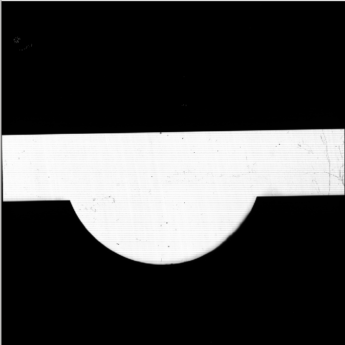
- "Odd-even effect": Alternate rows in the GNIRS science array have gains that differ by approximately 10 percent, which results in a high frequency "fuzz" in the raw spectra of continuum sources, flat fields, etc. (spectra run vertically on the array). This flat field, taken in imaging mode with the long blue camera, illustrates the effect. As long as the science spectra and the flat fields are not saturated, the fuzz is removed by flat-fielding.
- Electronic pattern: Like NIRI, GNIRS' GNAAC controller often superimposes vertical striping, horizontal banding, and small numerical offsets on the data. Occasionally more "random" patterns (e.g., stipple) are present. In the cases of striping, banding, and offsets, a python routine under development, cleanir, originally written for NIRI, is available and has proven to be effective at removing the patterns. Common uses of cleanir with GNIRS files are 'cleanir -rq filename.fits', 'cleanir -fq filename.fits', and 'cleanir -rqf filename.fits'. For other usages see the cleanir web page above. The nvnoise task in the GNIRS IRAF package can also be used. Here is an example of a raw file showing some pattern noise, and the same file after cleaning (in this case using nvnoise).
- Persistence: Signal or background that fills a substantial fraction of the array well capacity is likely to lead to persistence. This is a common phenomenon with InSb detectors (e.g. Campbell & Thompson 2005). For example, the acquisition of a faint target, which may utilize exposures that half-fill the array with background radiation produces a faint image of the imaging keyhole on the array in subsequent frames, often most easily seen in a subtracted pair of images. Likewise the spectrum of a bright calibration star will leave a faint spectrum on the array. The persistence fades away fairly rapidly. Science data are obtained in an ABBA pattern; a linear decrease in the persistence might be removed if data are obtained using that sequence. However, the drop-off is more like 1/time (see below) and thus in practice there is a faint positive residual image in the first subtracted pair (A-B) and a much fainter residual in the following one (B-A), and so they do not cancel. More detailed information follows.
A. Characterization of Persistence
- Persistence appears following any single exposure resulting in signal of ~ 1000 ADU or more. It increases linearly with signal above 1000 ADU. E.g., the persistence in a 120 second exposure immediately following a “flat” of 2000 ADU is ~4 ADU, for a “flat” of 3000 ADU the persistence is ~8 ADU, for a flat of 4000 ADU it is ~12 ADU. For a single flat of 1000 ADU it is ~0.
- Repeated exposures result in a somewhat larger persistence (by ~30 percent) in subsequent exposures. Repeated exposures at or slightly below the above threshold also create persistence.
- The “persistence current” decreases with time as ~ 1/t whether or not dark exposures (flushes) are taken. The persistence in a frame is then proportional to log (t2/t1), where t1 and t2 are the start and end times of the frame, both times measured from the end of the last exposure to cause persistence.
B. Effects of persistence on data and possible remedies/workarounds
Several types of observations result in signal levels that cause persistence and can deleteriously affect subsequent science frames.
- In the 1-2.5um region observations of bright standard stars (or bright targets) result in their spectra being imprinted on subsequent frames of faint science targets. The remedy for this is to observe the science target and standard star in different locations along the slit. The OT library templates are set up in this manner.
- In the L and M bands the sky background is bright enough to result in persistence, which is probably unimportant for L and M band science frames but could affect subsequent JHK faint source science spectroscopy frames. This can be mitigated by appropriate scheduling.
- Emission lines such as strong sky OH lines in the H and K bands and strong arc lamp lines can leave persistence on subsequent frames such as flats. This is difficult to avoid. The observing templates in the OT library are set up so as to obtain flats prior to arcs. The template flats are designed to produce large signals in order that the relative effect of the sky-line persistence is minimized.
- Observations of spectral flats result in persistence in subsequent frames. Because flats are "flat" in the spatial direction in most cases the persistence will subtract in subsequent A-B subtracted pairs. Problems may arise when a XD program is followed by a long slit program; this is a scheduling issue.
- The sky background in faint source acquisition frames can leave persistence in the form of an imprint of the keyhole on the first few science frames. Over much of the persistence region the effect goes away when one subtracts the negative spectrum from the positive spectrum (in A-B subtracted frames); but on the curved edges of the keyhole it does not. The acquisition exposure times in the OT library have been shortened to reduce this effect.
While the GNIRS team is making efforts to understand and avoid persistence as far as possible, it is an intrinsic property of the detector and cannot be avoided in all circumstances. The practical impact of low-level persistence on many science programmes may also be minimal. Users are encouraged to consider the possible effects on their science data and use the above information to plan accordingly.
- Flexure: As the telescope tracks across the sky the optics within GNIRS flex due to the change in direction of the gravitational force relative to the optics. This results in small wavelength shifts which are not steady but occasionally occur from one frame to the next, and it contributes to motion of the target relative to the slit. The latter, which is also due to flexure between the instrument and the wavefront sensor, requires occasional re-centering of the target in the slit (the frequency of this is discussed in the overhead section). The accumulated wavelength shift is typically ~0.5 pixels in an hour, but probably varies depending on telescope orientation. The shift can be measured by comparing the positions of sky lines in successive frames. The amount of degradation of resolution in one's data depends on the slit width (always at least 2 pixels) and on whether the spectra are shifted prior to summing them.
- Spectral FWHM of GNIRS+AO observations: Typical spectral FWHMs measured with GNIRS+Altair and the 2 pixel-wide slit during commissioning were around 3-4 pixels rather than the optimal 2 pixels. Because of the complexity of the optics in GNIRS we did not expect diffraction-limited performance.
- Short Camera ghosting: One of the lenses of the short red camera has no anti-reflection coating. In some configurations using that camera (in long slit mode) a ghost spectrum, roughly 5% of the intensity of the true spectrum has been observed horizontally offset from but parallel to the true spectrum, and also offset vertically in wavelength coverage. Similar ghosting, but at the 1% level, has been observed in the short blue camera in long slit mode when used with the 111 l/mm grating at certain wavelengths. In both cases the offset of the ghost spectrum from the true spectrum varies with the location of the true spectrum. For point sources, as long as the ghost does not closely coincide with the A or B spectrum of the target, the ghosting is harmless. Ghosting does have the potential to slightly interfere with L or M band observations of extended sources.
- ND100X+H2 ghosting: Bright-target acquisitions using the ND100X+H2 filters exhibit a comet-like tail which extends ~20 pixels above the target with a strength ~3% that of the target.
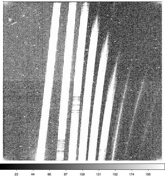
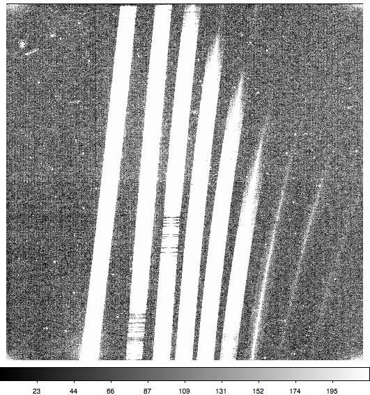
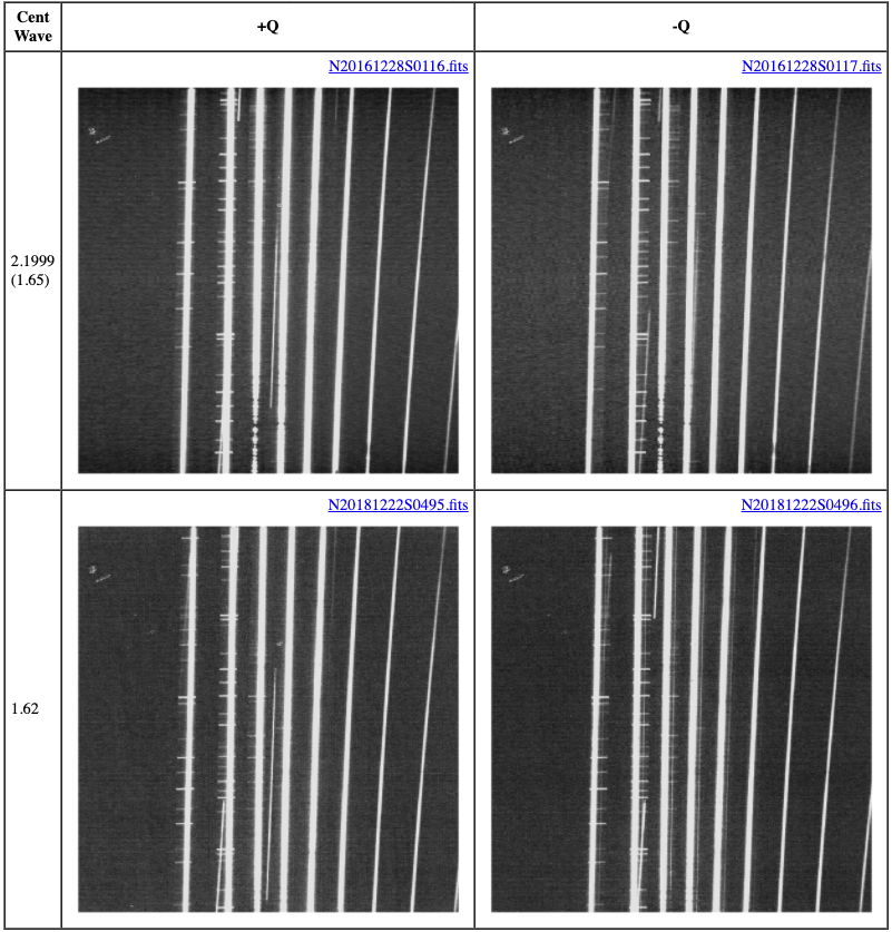
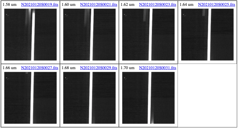
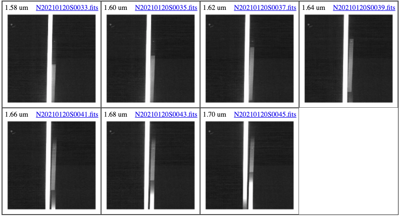
- Contamination GNIRS Short Blue camera + 111 l/mm grating + SXD cross disperser: The figure below shows an arc taken with the configuration mentioned and with a central wavelength of 1.62 um with the contaminants marked in green (note that the two lines marked in the upper left appear to be in the correct place, but they are not). It has been estimated that these reflections are ~0.4% of the primary signal. As a supplementary material, you can find the following data, which is taken with the same GNIRS configuration: The arcs taken with different order-sorted filters. Flats with the same filters. Telluric standards taken with the same configuration (central wavelength in the left column). Flats with the X order-sort filter at different wavelengths. Flats with the J order-sort filter at different wavelengths.
 |
- Slit length with Long Red camera: The current optical alignment inside GNIRS combined with the current version of the GNIRS control software does not allow simultaneous availability of the full length of the long slit (49") with both the long blue and long red cameras. We have opted to make the full long slit available with the long blue camera. With the long red camera the slit length is then ~45". If it is scientifically important for your program to have the full 49" slit length available for 3-5 micron spectroscopy, contact one of the GNIRS scientists assigned to the instrument.
- Bad Pixels: The GNIRS detector contains a few small regions of bad pixels. The bad pixels lie between the XD orders in the most heavily-used low-resolution XD modes (0.05"/pix + 10 l/mm and 0.15"/pix + 32 l/mm). However, the exact placement of the orders in the higher-resolution modes depends on the grating central wavelength. If the presence of these bad pixels could affect your science in these modes, please advise your contact scientist as you prepare your phase II observations. The CS will be able to take arc spectra that show exactly where the bad pixels will lie, and help you adjust your central wavelength to avoid them.
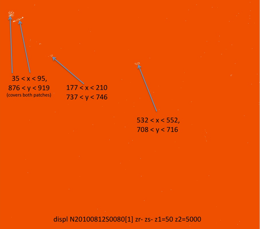
- Issue with upper right quadrant of the GNIRS detector: GNIRS recently began showing an issue that affects every 8th column on the top right quadrant of the detector, an issue that impacts all GNIRS modes (see images here). This issue first appeared on the 25th of October, 2022. Investigations to mitigate or fix the issue are currently ongoing. For the time being, PIs are advised to consider all pixels associated with these columns as bad pixels and not to use them for science and/or calibrations. A new bad pixel mask that masks every 8th column in the upper right quadrant in addition to the previously known bad pixels can be downloaded here. Note that this bad pixel mask is for use with Gemini IRAF, the equivalent BPM has been archived for DRAGONS.