Announcements
This section mainly describes how to prepare and check GMOS observations. Setting up acquisition and observing sequences at Phase II is not intuitive until one is quite experienced (and maybe even not then). An important key to successful observation preparation is starting from the GMOS OT Library. Preparing observing sequences involves much more than setting up the observation of the target; the complete observing sequences must include "acquisition observations" (e.g., for finding the target and putting it in the spectrograph slit). In addition, observations of telluric standards and/or flux standards, flat field calibrations, biases, and and arc lamps for wavelength calibration are usually needed.
Imaging Observing Strategies
The gaps between the three detectors in GMOS-S cause gaps in the imaging field about 4.9 arcsec wide. For GMOS-N, the inter-chip gaps between the three Hamamatsu detectors are 0.5 arcsec wider (5.4 arcsec). If continuous coverage of your field is needed, you will need to obtain multiple exposures and dither between the exposures. Due to additional bright columns at either side of the chip gaps, a minimum dither step of 10 arcsec in the X-direction (p-direction on the OT) is recommended. Please also note the updated recommendations on dither strategies to deal with the GMOS-N and GMOS-S detector artifacts.
(The gap width for the old GMOS-N e2v DD devices was 2.8 arcsec, and the recommended minimum dither step in X-direction 5 arcsec.)
For unbinned observations the pixel scale is 0.0807 arcsec/pixel (GMOS-N Hamamatsu) and 0.080 arcsec/pixel (GMOS-S Hamamatsu). (The pixel scale of the old GMOS-N e2v DD devices was 0.0728 arcsec/pixel.) If you are requesting imaging in image quality 70-percentile or worse, consider binning the CCDs 2x2 giving an effective pixel scale of 0.161 arcsec/pixel (GMOS-N) and 0.160 arcsec/pixel (GMOS-S). This cuts the overheads from the readout from ~83 sec to ~24 sec per frame(*).
The original GMOS EEV CCDs had strong fringing in the z' and i'-filters. The peak-to-peak amplitude was about 5% for the z'-filter. The new GMOS-N and GMOS-S Hamamatsu CCDs have less fringing in both the i' and z' filters. The peak-to-peak amplitude is about 2.5% for the Y-filter. For sparsely populated fields, fringe frames can be constructed from the science images. For crowded fields or extended objects, you may consider obtaining additional sky observations for the construction of fringe frames. Further information about fringing can be found here. To construct a reasonably good fringe frame you will need a minimum of six dithered science exposures.
Are the Baseline Calibrations sufficient for your program? If you need photometry to better than 5%, you will need to add standard stars to your observations to determine extinction. Photometry with the GMOS Hamamatsu detectors is complicated by the fact that the three CCDs in each of the GMOS detector arrays have different quantum efficiency characteristics. The implications for photometry are outlined here, together with an overview of calibration options and recommended observing strategies.
(*) Final characterization of the read-out overheads for the GMOS-N Hamamatsu detectors is ongoing.
Long-slit Observing Strategies
Long-slit
The gaps between the three detectors in GMOS cause gaps in the spectral coverage, see the example. The size of the gaps in wavelength space depends on the grating used, but is typically a few nanometers. If continuous spectral coverage is essential for your program, consider using two central wavelength configurations of the grating. The recommended wavelength dither steps for the Hamamatsu detectors are >~ 20 nm (R150 grating), >~7.5 nm (R400 grating), and >~ 5 nm for all other gratings. Please also note the updated recommendations on dither strategies to deal with the GMOS-N and GMOS-S detector artifacts.
The GMOS long-slits have bridges that cause gaps in the spatial coverage, see the example. The bridges are approximately 5 arcsec wide (Hamamatsu) and 3 arcsec wide (e2v). If continuous spatial coverage of your long-slit observations is needed, consider dithering in the Y-direction (q-direction on the OT). A minimum dither step of 5 arcsec is recommended.
If you are requesting long-slit observations in image quality 70-percentile or worse, consider binning the CCDs by two in the spatial (Y) direction giving an effective pixel scale of 0.1614 arcsec/pixel at GMOS-N and of 0.160 arcsec/pixel at GMOS-S.
You may also consider binning in the spectral (X) direction depending on how well-sampled your spectra need to be. For example, with the B600 grating and a 1" slit, the resolution is about fwhm=0.54 nm, which is equivalent to ~10 unbinned pixels (Hamamatsu) or 12 unbinned pixels (e2v). Use the grating information to derive this information for other configurations.
If your science target cannot be detected in imaging mode in one of the GMOS filters in about 1 min of exposure time (corresponding to 2-3 min of through-slit exposures), you will need to define a blind offset acquisition. Under average conditions (IQ85, CC70, SB80, airmass 1.5), point sources brighter than 21 mag (Vega) in any of the g'r'i'z' filters are typically suitable for direct acquisitions. For fainter or extended sources you will need to supply coordinates for a nearby brighter target (R<19 mag. and preferably a point source) and accurate offsets between that brighter target and your science target. For GMOS-S, the accuracy of blind offsetting is better than 0.1 arcsec for offsets less than 20 arcsec. For GMOS-N, the accuracy is better than 0.1" independent of distance. For the blind offsetting to work it is essential that the same guide star can be reached for the bright object and the science target.
If your science target is fainter than about R=18, you will have to supply a finding chart at the time of Phase II submission.
If you are observing very faint objects in the red, you may want to consider if your program would benefit from using GMOS in Nod-and-Shuffle mode.
Are the Baseline Calibrations sufficient for your program? If you need accurate telluric line removal, you will need to add telluric standard stars to your program. If you need radial velocity standards, then these need to be added to your program.
MOS Mask Preparation and Observing Strategies
Mask Preparation
The GMOS MOS masks must be designed either from images acquired with GMOS, or from object catalogs with very accurate relative astrometry. MOS PIs are encouraged to submit their mask designs as early as possible in order to increase the chance that the MOS observations will be completed. Detailed information on the deadlines for the mask design submission for GMOS-S and GMOS-N masks can be found in the Phase II instructions for the current semester.
Mask design from new GMOS pre-imaging
The pixel positions of the spectroscopic targets are obtained from a GMOS image. Due to distortions over the GMOS field of view, this image has to be taken with the same pointing and orientation on sky as planned for the MOS observations. If no prior GMOS image is available, PIs can request pre-imaging in queue mode prior to the classical or queue mode MOS spectroscopic observations. Observing time for pre-imaging will be charged against the program's allocated time and must be requested during Phase I. The observations should be defined as part of the Phase II process as early as possible during the semester, so that the images can be obtained once the target field becomes accessible. PIs may want to access carefully the observing conditions needed for the pre-imaging. Requesting very good observing conditions may lower the chance of getting pre-imaging data early during a semester, and therefore negatively impact the overall chance of getting the MOS observations completed within a given semester.
Mask design from previous GMOS images
Imaging obtained with one GMOS in a prior semester may be used for the mask design for the same instrument if the observations were taken with exactly the same pointing and orientation on the sky as is planned for the MOS observations. For a given pointing and orientation, the location of the OIWFS patrol field on the sky depends on whether GMOS is on the up-looking port or one of the side-looking ports on the telescope. Imaging data obtained with GMOS on the up- or side-looking port may be used for a mask design for the other type of port only if a suitable guide star is available without changing the pointing and orientation of the field on the sky. GMOS North was on the up-looking port in 2001B, and has since been on the side-looking port. GMOS South is on the side-looking port. If you are in doubt about whether existing pre-imaging can be used for your mask design, please contact the Gemini HelpDesk.
Existing images from other telescopes or the other GMOS instrument
GMOS-N images cannot directly be used for GMOS-S mask designs and vice versa. If a PI has prior imaging from the respective other GMOS instrument or other telescopes, pre-imaging with the GMOS instrument used for the MOS observations is required. However, if there are existing images of the field, it may be possible to base the mask design on new pre-images obtained with quite short exposure times and/or in worse seeing conditions than needed for the spectroscopy. If the GMOS images contain a sufficient number of objects (> 50) with good signal-to-noise then these objects may be used to "boot-strap" the pixel positions of the science targets. This would be useful if, for example, the relative astrometry provided by the WCS is not accurate enough to construct a reliable object catalog.
Mask design from a catalog
The mask is designed from accurate relative coordinates (RA and Dec) for the spectroscopic targets from a catalog. In this case, known transformations are used to calculate the GMOS pixel positions from these coordinates. The PI must have an object catalog with accurate relative coordinates for spectroscopic targets and alignment stars. It is crucial that all coordinates in the object catalog be given in the same astrometric system, as systematic offsets between science targets and acquisition targets for example will produce a fatally flawed MOS mask. In most cases these coordinates should be known with a relative accuracy < 0.1 arcsec. Gemini recommends that masks with slit widths narrower than 1 arcsec be designed from GMOS direct imaging rather than solely from object catalogs. The PI must also create a "pseudo-GMOS" image of the field, using the gmskcreate task available as part of the Gemini IRAF package. This pseudo-GMOS image must be submitted via the OT along with the mask design as it is required during the mask checking process. This image is created from a PI-supplied image taken with another telescope and the gmskcreate task transforms that image onto GMOS pixels when you specify fl_getim=yes. As with MOS masks designed from GMOS direct imaging, the PI designs the mask for a specific field center and position angle on the sky. Once the mask design is submitted these cannot be changed, therefore the PI must verify that a suitable guide star exists for that field center and position angle. The OT can be used for this. The MOS observations defined in the OT must use the same coordinates and position angle as those used for the mask design.
MOS Observing Strategy
- Wavelength dithers: The gaps between the three GMOS detectors cutout small wavelength intervals (grating dependent) from the spectra. If continuous spectral coverage is important for you, then at least two sets of observations with slightly different wavelengths are needed. The recommended minimum shifts are ~20nm for the R150 grating, ~7.5nm for the R400 grating, and ~5nm for all other gratings. Please also note the updated recommendations on dither strategies to deal with the GMOS-N and GMOS-S detector artifacts.
- Spatial binning: If you are requesting MOS observations in image quality 70-percentile or worse and your slitlets are longer than 3 arcsec, consider binning the CCDs by 2 in the spatial (Y) direction giving an effective pixel scale of 0.16 arcsec. If you are using very short slits (3 arcsec or less), then spatial binning is not recommended (not even for nod&shuffle mode).
- Spectral binning: Consider spectral binning (X direction) if the spectral resolution can be lower than that provided by the grating and the slit width. For example, with the B600 grating and a 1" slit, the resolution is about fwhm=0.54 nm, which is equivalent to ~11 unbinned pixels. Use the grating information to derive this information for other configurations.
- When to use Nod&Shuffle mode: If you are observing very faint objects in the red or need slits that are very densely packed, your program could benefit from Nod-and-Shuffle mode. The overheads for Nod-and-Shuffle are significant, but can be minimized by nodding along the slit, keeping the science target(s) in the slit(s) for both the A-position and the B-position. Small nod distances have lower overheads than large nod distances. Very small nod distances (< 2arcsec) can further reduce the overheads by employing electronic offsetting. If the program requires nodding off to sky, ie. not having the science target(s) in the slit(s) in the B-position, nodding in the q-direction as defined in the observing tool has the lowest overheads.
- Nod&Shuffle offsets: MOS Nod-and-Shuffle programs which are nodding along the slit need to make sure that the slit length specified in GMMPS is compatible with the total offset distance defined in the Observing Tool's Nod-and-Shuffle component. GMMPS displays the correct numbers when loading the ODF mask design file. Nod-and-Shuffle MOS observations should always use symmetric offsets about (0,0) in the Observing Tool.
- Calibrations: Are the Baseline Calibrations sufficient for your program? If you need accurate telluric line removal, you will need to add telluric standard stars to your program, or if possible you can add a few blue objects to your mask design. You will have to be sure that these stars are spread across the CCDs so that they cover the spectral range sampled by your observations. If you need radial velocity standards, these need to be added to your program. In most cases, the MOS baseline standard star should be taken at three central wavelengths to fully sample the spectral range covered by slits at the left and right side of the slit placement area. The grating-dependent offset recommendations are:
- R400: science central wavelength +/- 150 nm
- B480: science central wavelength +/- 125 nm
- B600: science central wavelength +/- 100 nm
- R600: science central wavelength +/- 100 nm
- R831: science central wavelength +/- 80 nm
- B1200: science central wavelength +/- 30 nm
- R150: no offset needed
- Acquisition: 2-3 stars are centered in 2x2 arcsec acquisition boxes. With pre-imaging 2 alignment stars are needed; with catalog masks 3 stars are required. The acquisition objects should be bright enough to give a good S/N (larger than 200) in a 30s imaging exposure with GMOS. They should also be faint enough that the spectra of them do not significantly saturate the CCDs during the science exposures. To ensure efficient acquisition, point sources with V magnitudes in the interval 16 mag to 20 mag are recommended for observations with grating R150. For observations with gratings B600 and R400, it is recommended to use point sources with V magnitudes in the interval 15 mag to 20 mag. Fainter acquisition objects may be used, but additional time should be budgeted for target acquisition.
- Guiding: For catalog masks, please make sure that there is an appropriate guide star available for the coordinates and PA of the mask design. Check also that this guide star is not also one of the mask acquisition stars!
- Fringing: GMOS CCDs show fringing in the far red. If the objects are faint and the spectral region of interest is located where there is fringing, good sky subtraction can be obtained by observing the objects in at least two positions along the slit. In this way, one can use one image to subtract the sky from the other image and obtain two sky subtracted spectra of the objects. This is a primitive way to do Nod & Shuffle. An alternative is to use N&S.
IFU Observing Strategies
The gaps between the three detectors in both GMOS cause gaps in the spectral coverage, see the data examples. The size of the gaps in wavelength space depends on the grating used, but is typically a few nanometers. If continuous spectral coverage is needed, the recommended minimum shifts are ~20 nm for the R150 grating, ~7.5 nm for the R400 grating, and ~5 nm for all other gratings. Please also note the updated recommendations on dither strategies to deal with the GMOS-N and GMOS-S detector artifacts.
The width of each fiber in the IFU is only 5 unbinned pixels. Thus, it is recommended to always have the Y-direction of the detectors unbinned. The spectral resolution of the IFU is equivalent to a slit with 0.31 arcsec width (3.88 unbinned pixels for Hamamatsu, 4.26 unbinned pixels for e2v), thus you may consider binning in the spectral direction if your object is very faint.
You will have to decide if your science targets are best observed in IFU 2-slit mode or IFU 1-slit mode. The 2-slit mode gives you a larger field on the sky at the expense of spectral coverage. The 1-slit mode gives you larger spectral coverage, but half the field of view on the sky compared to the 2-slit mode. In 2-slit mode you will have to use one of the color filters in order to avoid overlap between the spectra, see the spectral overlap page for details. In 1-slit mode you may have to use a filter to avoid 2nd order contamination.
In 1-slit mode the central wavelength you specify will be interpreted as the desired wavelength at the center of the detector array. In 2-slit mode, the central wavelength you specify will be the wavelength at the location of the two pseudo-slits.
If your science target cannot be detected in imaging mode in one of the GMOS filters in about 1 min of exposure time (corresponding to about 3 min of through-IFU exposures), you will need to define a blind offset acquisition. Under average conditions (IQ85, CC70, SB80, airmass 1.5), point sources brighter than 21 mag (Vega) in any of the g'r'i'z' filters are typically suitable for direct acquisitions. For fainter or extended sources you will need to supply coordinates for a nearby brighter target (R<19 mag. and preferably a point source) and accurate offsets between that brighter target and your science target. The accuracy of blind offsetting is better than 0.1 arcsec for offsets less than 20 arcsec. For the blind offsetting to work it is essential that the same guide star can be reached for the bright object and the science target.
If your science target is fainter than about R=18, you will have to supply a finding chart at the time of Phase II submission.
Are the Baseline Calibrations sufficient for your program? If you need accurate telluric line removal, you will need to add telluric standard stars to your program. If you need radial velocity standards, these need to be added to your program. Also if you need very accurate velocity calibration and you are observing in the blue where not many skylines are available from which to bootstrap your daytime CuAr, you may need to request CuAr calibrations be taken on the sky with your science observation. On-sky arc lamp exposures for setups which do not cover at leat the 5577 A sky line are provided as part of the baseline calibrations (details can be found here).
IFU Target Acquisition and Observation Definition
IFU Target acquisition is done by taking a GMOS image of the field using the sub-region of the CCDs that contains the IFU fields. An IRAF task in the Gemini package can overlay the IFU fields on the image and calculate the offsets to the desired position in the IFU field-of-view. Another task does rapid IFU image reconstruction to verify the placement of the target in the IFU. The following information is needed to define an IFU observation:
- One-slit or two-slit mode. If in one-slit mode, then one can choose which slit to use (IFU Right Slit (Red) recommended for both GMOS-N and GMOS-S).
- Coordinate to be centered in the desired IFU field.
- Position angle (PA) to track. Note that the long axis of the Object field changes by 90 degrees between one and two-slit modes.
- Whether beam-switching is needed
- Blocking filter
- Grating
- Central wavelength at the position of the pseudo-slits.
- CCD binning (no binning recommended).
- Exposure time
Spectral Overlap in 2-Slit Mode
In one-slit mode the grating and filter combinations may be selected as for long slit spectroscopy.
In two-slit mode the broad-band filters can be used to prevent the two banks of spectra from overlapping on the detector. The useful combinations of gratings and filters that allow the use of two slits with no or minimal overlap are given in the table below. The calculated separations between the slits in unbinned pixels for the various grating/filter combinations are also given. Differences in the slit separations are due to anamorphic magnification. For most of the configurations below, the complete filter passband fits on the detector for both slits (typically with a few nm lost due to overlap at the center). With the B600 (or R600) grating + g filter at 475nm, 11.5nm of the g passband is lost at either end of the detector, so the blue slit has slightly less blue coverage and the red slit slightly less red coverage. In general, one should set the grating central wavelength to that of the filter for two-slit mode (+/- 11.5nm for B600+g), to avoid losing spectral range at the ends of the detector unnecessarily. Small adjustments may be needed to account for the CCD gaps. For the R150 + GG455, a central wavelength of ~680nm will cover roughly 460-900nm at both slits (truncating the very red end of the red slit; longer settings will reach >=1000nm at the expense of the blue end of the blue slit).
Note that with the R150 grating in 2-slit mode, there is a small amount of second order contamination from the blue slit overlapping the red slit (eg. for a central wavelength of 630nm, this peaks at the level of ~4%, dying away in the red). See the gratings and GMOS-N and GMOS-S filters page for more information on GMOS gratings and filters.
R150 zero-order contamination in 2-Slit Mode
When using the IFU 2-slit mode together with the R150 grating, a part of the spectrum from the blue IFU pseudo-slit is affected by a zero-order contamination from the red IFU pseudo-slit. The affected wavelength region has been measured based on extracted, wavelength-calibrated, and distortion-corrected arc frames observed with GMOS-N and GMOS-S for different central wavelength settings. The pseudo-slits are not perfectly straight, but show slight positional shifts between individual fibers and between fiber blocks. Consequently, the effective wavelength of the contamination in the blue-slit spectrum shows small variations from fiber to fiber. The plot below illustrates the total width of the zero-order contamination in wavelength space after summing over all fibers from the blue pseudo-slit. The central wavelength setting of each data set is marked in the legend. (The absolute and relative scale of the counts in this plot is arbitrary.)
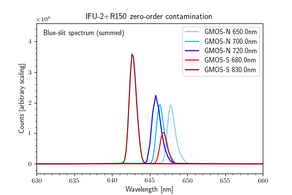
The data sets show that the effective wavelength of the zero-order contamination is similar for GMOS-N and GMOS-S. The longer the central wavelength setting, the shorter the effective wavelength of the contamination. Using a large central wavelength dither can potentially help with mitigating the effect from the contamination in the combined spectra. However, the benefit from large central wavelength dithers needs to be evaluated against the fact that unusually large or short central wavelengths will shift a part of the R150 wavelength coverage beyond the borders of the detector.
Nod and Shuffle Observing Strategies
The recommendations and performance numbers given in this section are based on observations done during the commissioning and System Verification in August and September 2002. For the Hamamatsu CCDs, which have a higher sensitivity in the red, the considerations below still apply, however the exposure times may be ~1/3 shorter.
- Recommended Exposure Times: Choosing the best exposure time for Nod & Shuffle observations is highly dependent on the stability of the current cloud cover conditions. There is a trade-off because shorter exposure times, while yielding more accurate sky-subtraction also lead to significantly increased overheads. During Commissioning and System Verification for Nod & Shuffle it was determined that an exposure time of A = 60sec gave acceptably low sky-subtraction residuals for photometric or nearly photometric (CC = 70%) and relatively stable sky conditions. For highly variable sky conditions or heavier cloud cover (CC = 90% or Any) an exposure time of A = 60sec gave unacceptably high residuals and we recommend a shorter exposure time, e.g. A = 30sec.
- Sky subtraction and Nod & Shuffle -vs- Classic GMOS Spectroscopy: Nod & Shuffle gives the possibility of eliminating systematics from the sky subtraction, even in the presence of very strong sky lines. The advantage of Nod & Shuffle is largest in the red, due to the many strong sky lines. By eliminating the systematics from the sky subtraction, Nod & Shuffle makes it possible to combine spectroscopic observations to reach total exposure times of many tenths of hours without being affected by systematic sky residuals. It has been demonstrated that with total exposure times of 28 hours it is possible to determine redshifts from absorption lines of objects as faint as i'(AB)=24.7 mag. For exposure times of a few hours and fairly bright objects, typically i' brighter than 20-21 mag, the advantage of Nod & Shuffle is smaller. However, if you are concerned about getting high signal-to-noise spectra and are studying faint absorption features, you may still want to consider Nod & Shuffle. Example longslit spectra taken with Nod & Shuffle illustrate these points.
- GMOS Integration Time Calculators The GMOS North and South ITCs do not account for systematic uncertainties in the subtraction of bright skylines, and as such is quite easily adapted for estimating realistic sensitivities using Nod & Shuffle. All one needs to do is to set the sky aperture to 1 times the target aperture in the Analysis Method under Details of Observation instead of using the default sky aperture of 5 times the target aperture.
Overheads
For the Phase I observing proposals that are not using Nod-and-Shuffle and do not require very detailed timing, you can use the telescope setup times given below, plus 2 min per exposure to cover readout, filter changes etc.
When using Nod-and-Shuffle, additional overheads apply: these overheads should be added to the overheads from the telescope setup and the readout etc., whenever Nod-and-Shuffle is used.
For more exact calculation of the overheads where these are critical to your observing program (for example time-resolved observations), the detailed listings on this page may be used. The detailed overhead information is also useful for the Phase II planning of your observing program. The various overheads can be broken into the following categories:
- Telescope setup time
- GMOS configuration time
- Readout time
- Telescope offsetting time
- Calibrations
- Additional nod-and-shuffle overheads
Telescope setup (acquisition) time
The setup times below include slewing to a new target, starting guiding, and accurately centering objects on slits (if appropriate).
| GMOS mode | Setup time |
| Imaging | 6 min |
| Long-slit | 16 min |
| IFU | 18 min |
| MOS | 18 min |
Applicants for GMOS time should allow for one acquisition for approximately every 2 hours observed (including overheads and calibrations). Shorter observations may also be split in order to accommodate them in the queue planning.
The acquisition times listed above are based on average statistics from the last two years of GMOS observations. Note that if acquiring particularly faint targets requiring long exposure times (> 2 min) the actual acquisition times will be longer. PIs should take this into account when filling out their Phase I proposals and Phase II programs.
GMOS configuration times
Below are listed approximate configuration times for various components within GMOS (the exact times depend on the details of the positions between which a particular component is being moved). It is possible (and usual) to reconfigure GMOS while slewing to a new target, but it is not currently possible to reconfigure GMOS while reading out the detector. This is a limitation of the current software that is used to execute sequences.
| GMOS component | Config Time |
| Filter change | 20 sec |
| Grating change | 90 sec |
| Mask move in or out | 60 sec |
Readout times
Below are listed the readout times, including the overhead added by the sequence executor software, which is used to execute sequences. It is unfortunately not possible to reconfigure GMOS, dither the telescope position or begin setup on the next target during readout.
The table shows the overheads for the GMOS-N E2V DD detectors (6-amplifier read out) and GMOS-S Hamamatsu detectors (12-amplifier read out). Please note that the GMOS-N E2V DD detectors were replaced with Hamamatsu CCDs in March 2017. Until the measurement of the new overheads for the GMOS-N Hamamatsu detector array (12-amplifier read out) is complete, PIs should assume the GMOS-S (12amp) overheads.
| ROI* | Binning | Read speed | Readout Time (s) | |
| GMOS-N (6amp) | GMOS-S (12amp) | |||
| Full frame | 1x1 | slow | 76 | 83 |
| Full frame | 1x1 | fast | 36 | 35 |
| Full frame | 1x2 | slow | 46 | 41 |
| Full frame | 2x1 | slow | 49 | 50 |
| Full frame | 2x2 | slow | 31 | 24 |
| Full frame | 2x2 | fast | 20 | 11 |
| Central spectrum** | 1x1 | slow | 25 | 20 |
| Central spectrum | 1x2 | slow | 18 | 11 |
| Central spectrum | 2x1 | slow | 18 | 15 |
| Central spectrum | 2x2 | slow | 14 | 9 |
| Central spectrum | 4x4 | slow | 11 | 4 |
| Central spectrum | 4x4 | fast | 11 | 3 |
* For more details on Regions of Interest (ROIs) see the GMOS OT component page.
** The "Central spectrum" ROI corresponds to the central 1024 (unbinned) rows of the detector array in the spatial direction and the full width of the array in the spectral direction.
Telescope offsetting time
The time to offset the telescope as part of a dither sequence is currently ~7s (from the time of turning off guiding at one position to guiding at the next position). At present it is not possible to offset the telescope while reading out the detector when these operations are parts of a sequence.
Configuration for Calibrations
A portion of the overhead for taking calibrations is the time it takes to move the science fold mirror, which sends the beam either from the sky or from GCAL into GMOS. Again, when using the sequence executor to run sequences, this move cannot be done while reading out the detector array.
With GMOS on side port 5, the relevant science fold moves take about 20 seconds each. Therefore the total overhead to move to and from the calibration position is about 40s. (This does not include the time to actually take the calibrations).
Additional Observing Overheads with Nod & Shuffle
When observing with Nod & Shuffle the same GMOS observing overheads as for classical long-slit and MOS spectroscopy target acquisition and detector readout are still applicable. However, there are additional Nod & Shuffle overheads which are substantial and must be considered in the Phase I observing proposal. The "rule of thumb" given below can be used for a large fraction of Nod & Shuffle programs. Details are also given, in case the "rule of thumb" does not apply to your program.
- Rule of thumb. If you are nodding along the slit and use nods of less than 10arcsec but greater than 2arcsec, the approximate time required to get 1800sec open shutter time (A-position plus B-position) is 2200sec, plus time for acquisition and readout. For nods with a total distance of 2arcsec or less one can elect to use electronic offsetting of the OIWFS, in which case this time is reduced to 2000 sec.
- GMOS Nod & Shuffle overheads are defined as the time per cycle that the shutter is closed. This excludes readout and target acquisition. This also assumes nodding along the slit, meaning all open-shutter time is spent collecting data on the target.
- Example 1: Exposure time A = 60sec, Overhead = 24sec, nodding along the slit.
Effective overhead (time spent not observing target) per cycle is 24sec, or 24/(60+60) = 20% - Example 2: Exposure time A = 30sec, Overhead = 24sec, nodding along the slit.
Effective overhead (time spent not observing target) per cycle is 24sec, or 24/(30+30) = 40% - Example 3: Exposure time A = 60sec, Overhead = 24sec, nodding off to sky.
Effective overhead (time spent not observing target) per cycle is 84sec, or (24+60)/60 = 140%
- Example 1: Exposure time A = 60sec, Overhead = 24sec, nodding along the slit.
- Additional overheads above the 24 sec depend on the size and the direction of the telescope nod, and appear to be limited by the speed at which the GMOS OIWFS moves into position. Nods in the q-direction appear to be much more efficient (less overhead) than nods in the p-direction (perpendicular to the slit).
- Nods in the q-direction can be approximated as adding another additional 1sec of overhead per cycle for every 15 arcsec of distance, eg. a nod of q=30 arcsec gives an overhead of 26 sec per cycle.
- Nods in the p-direction can be approximated as adding another additional 0.6sec of overhead per cycle for every 1 arcsec of distance, eg. a nod of p=30 arcsec gives an overhead of 42 sec per cycle. It is strongly recommended to nod in the q-direction (i.e., parallel to the slit).
- Very small absolute nod sizes (< 2.0arcsec) can take advantage of electronic offsetting of the OIWFS. In this case the GMOS OIWFS does not actually move, only the position of the spots on the wavefront sensor is electronically shifted. The effective overhead per cycle is reduced to 13.5 seconds, so observations which can tolerate such small nods are encouraged to use this feature.
GMOS OT Details
This page explains how to configure the Gemini Multi-Object Spectrographs (GMOS) in the Observing Tool. There are separate components and iterators for GMOS-N and GMOS-S (because the list of filters, gratings etc may differ):
- GMOS Component - to define 'static' configurations
- GMOS Iterator - to sequence different instrument configurations
- GMOS OIWFS (on-instrument wavefront sensor) field of view - displayed in the position editor
GMOS Component
The detailed component editor for GMOS is accessed in the usual manner, by selecting the GMOS component in your science program. Select the GMOS-N component if your program is scheduled for Gemini-North; select GMOS-S component if your program is scheduled for Gemini-South. The example below shows GMOS-N component. This window looks similar for GMOS-S.
.png)
Selecting a filter
The filter is chosen by clicking on the pull down list (i.e. the down-pointing arrow) and selecting the desired filter. The filter names match those listed on the GMOS filter pages. In spectroscopic mode, all filters can be used as blocking filters as required by your science program. There is no requirement to use a filter in spectroscopic mode.
Setting the exposure time
The exposure time is set typing the number of seconds in the "Exposure Time" field. The exposure time must be a non-zero integer.
Selecting a disperser and the central wavelength
Choice of grating (for spectroscopy) or mirror (for imaging) is made by clicking on the pull down lists (i.e. the down-pointing arrows) and selecting the desired item. The grating names match those listed on the GMOS grating pages. If a grating is chosen, the grating central wavelength must also be set and the order chosen. Currently all gratings are only used in first order.
Selecting the CCD manufacturer
GMOS-S and GMOS-N were upgraded with red-sensitive Hamamatsu CCDs in 2014 and 2017, respectively. Therefore, the CCD manufacturer should be set to "HAMAMATSU".
Selecting a focal plane unit
Choice of one of the built-in focal plane units is made by clicking on the pull down lists (i.e. the down-pointing arrows) and selecting the desired unit. The built-in focal plane units include various longslits and the IFU. For imaging, the focal plane unit should be set to "None". For MOS observations a custom Mask Definition File (MDF) is needed. Select the custom mask MDF by clicking the "radio"-button. Then type the MDF label supplied from the Gemini Observatory for your observation(s) in the field to the right.
Note that the longslit length for nod-and-shuffle observations is approximately 1/3 of the regular longslit (to provide sufficient un-illuminated areas on the detector within which to shuffle the charge). Make sure that you have selected the correct slit for your observations.
If you display a view of the field with the position editor and have selected the "science area" button, then this will reflect the choice of focal plane unit (displayed as a blue box). Note that because of their small field of view, the two integral field unit 'apertures' can be quite hard to see. Currently, all custom mask MDFs are shown as the largest field of view within which slit-lets can be cut.
Setting the position angle
The facility Cassegrain Rotator can rotate the instrument to any desired angle. The angle (in conventional astronomical notation of degrees east of north) is set by typing in the "position angle" entry box. The view of the science field in the position editor will reflect the selected angle. Alternatively the angle may be set or adjusted in the position editor itself by interactively rotating the science field.
GMOS users may elect to use the average parallactic angle in order to minimize the effects of atmospheric differential refraction. This is strongly recommended for all long-slit observations where the position angle is otherwise unconstrained. When the "Average parallactic" option is selected, the nighttime observer will use the "Set To" drop-down menu to calculate the airmass-weighted mean parallactic angle. It is recommended that PIs set the PA to 90 for observations using the average parallactic angle and verify that a guide star is available. The OT will automatically search for the best guide star at PA=90 and PA=90+180. If no guide star is available with the OIWFS, the default guider should be changed to PWFS2, keeping in mind that flexure may require reacquisitions for observations longer than ~45 minutes. Note that the average parallactic angle option is only available for longslit and IFU observations.
Setting CCD readout details
Select the binning in the X and Y direction by clicking on the pull down lists (i.e. the down-pointing arrows). No binning (1), and binning by 2 and 4 are supported. For imaging mode, the binning in X and Y should be set identically. For the spectroscopic modes, binning in X is equivalent to binning in the spectral direction, while binning in Y is equivalent to binning in the spatial direction.
Select the desired read-out mode/gain combination. The available modes are those listed as suggested settings on the GMOS Detectors web pages. For the Hamamatsu CCDs twelve amplifier read-out is the default and the number of amplifiers is not user-selectable.
Setting Translation stage details
The GMOS detector is mounted on a translation stage to compensate for flexure. The default setting, "Follow in X and Y", currently gives the best flexure compensation for GMOS-N. For GMOS-S, the default setting is "Follow in X, Y and Z". For daytime calibration such as arcs and mask images taken when the telescope is stationary, the translation stage should be set to "Do Not Follow" for GMOS-N and "Follow in Z Only" for GMOS-S.
The DTA-X option allows the PI to shift the spectral image on the detector array by an integral number of unbinned rows, allowing for averaging of pixel features not adequately removed by flat fielding. The number of DTA-X pixels selected should be an integral factor of the detector y-binning to avoid shifting by partial binned rows. Note: DTA-X offsetting was implemented to aid in the suppression of linear charge traps affecting Nod & Shuffle data in the original EEV detectors. With the upgraded GMOS-N and GMOS-S Hamamatsu detectors DTA-X offsetting is no longer as advantageous.
Setting the region of interest (ROI)
The GMOS detector can be configured to either read out the full frame or read out a smaller region of interest. The default is to read out the full frame. To change this, click on the "Regions of Interest" tab and then click the "radio"-button on the preferred region of interest.
The GMOS-S and GMOS-N Hamamatsu detector arrays are 6144 pixels by 4224 pixels. The regions read out for the different choices of region of interest (ROI) are given in the table below as [x1:x2,y1:y2], where x1 and x2 are the starting and ending pixel in the X direction and y1 and y2 are the starting and ending pixel in the Y direction. The ROIs are given in unbinned pixels. All ROIs can be used with all binnings; the software takes care of any needed conversions. The table below also lists typical use for the different ROIs. Currently the chosen ROI is not visualized in the Position Editor.
| Name of ROI | [x1:x2,y1:y2] | Common use |
| Full Frame Readout | [1:6144,1:4224] | Most science observations. |
| CCD2 | [2049:4096,1:4224] | Longslit with color filters when useful wavelength range can fit on 2048 pixels. |
| Central Spectrum | [1:6144,1625:2648] | The central 1024 rows. Longslit spectra of point sources (standard stars). |
| Central Stamp GMOS-S Central Stamp GMOS-N |
[2923:3222,1987:2286] [2923:3222,1987:2294] |
The central 300pix x 300pix. Imaging of single standard stars. The central 300pix x 308pix. Imaging of single standard stars. |
Selecting the ISS port
The location of the GMOS OIWFS patrol field on the sky depends on which ISS port on the telescope has GMOS mounted. Normally GMOS is mounted on the "side-looking" ISS port. The OT has this selection as its default. It is important to make sure that the correct ISS port is selected for the current semester, since it affects whether the selected OIWFS guide star can be reached.
Nod-and-Shuffle specifications
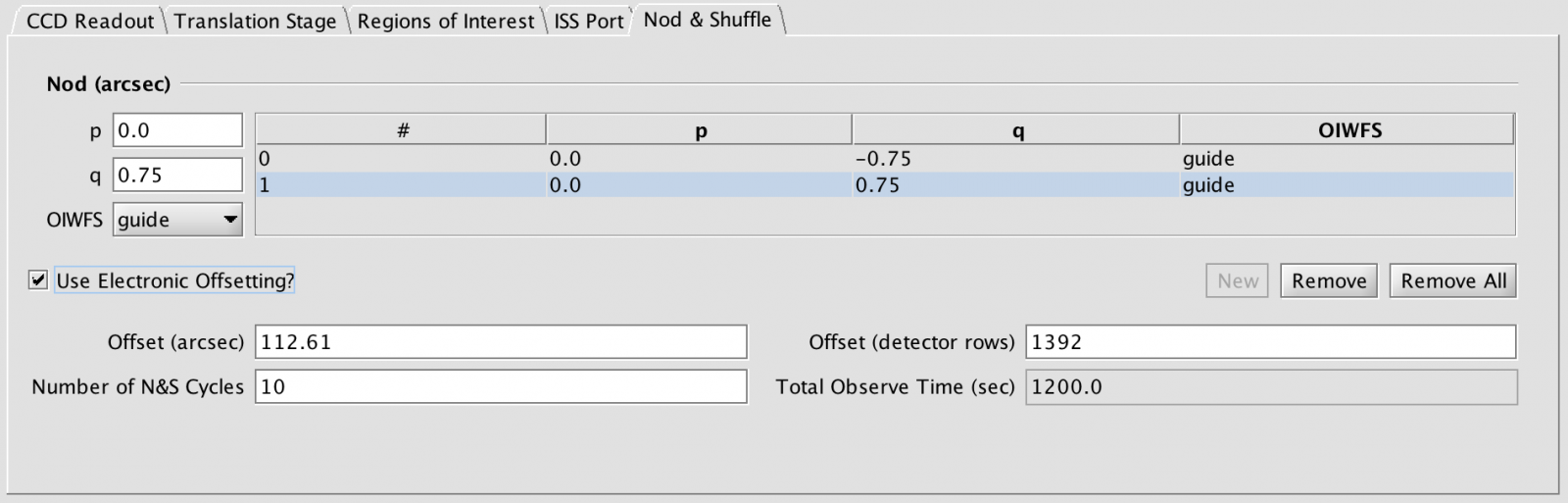
First you must select nod-and-shuffle mode using the radio-button in the upper right hand corner of the GMOS component. Once that is selected, the nod-and-shuffle tab becomes active. (Depending on the size of your window, you may have to use the arrows to the right of the tabs to locate it). The content of the nod-and-shuffle tab is shown below.
The following items need to be defined by the user:
- A valid nod-and-shuffle configuration has two offset positions. As default the first [p,q] offset position is set to (0,0) and the second to (0,10) arcsec. An offset in q means a nod along the slit, regardless of instrument rotation angle, giving the possibility of having the target on the slit for both nod positions.
- If the distance between the two nod positions is less than 2 arcsec then electronic offsetting can be used to reduce overheads (see below). When using electronic offsetting it is best to offset around (0,0) as in the example above. During electronic offsetting the telescope motion is compensated electronically so that the OIWFS probe arm does not have to move.
- Set the guide configuration as needed. You may guide at both offset positions, if the OIWFS probe arm can reach the guide star for both offset position. Or you may "freeze" the OIWFS probe arm on for position #1 (beam B) - usually only used if you are nodding off to sky rather than along the slit.
- Set the "shuffle". By default the shuffle offset is set to 1392 (112.61 arcsec) for the Hamamatsu detectors (1536 rows - equivalent to 111.67 arcsec - for the previous e2v detectors). This is appropriate for longslit observations. For the GMOS-S IFU the shuffle should be 256 rows. For MOS the "shuffle" must match the mask design. You can define the shuffle either in arcsec or in detector rows and the other is calculated automatically. The shuffle must be an integer number of rows in unbinned pixels; a warning is issued if the number of rows is not exactly divisible by the Y-binning. If the offset is entered in arcseconds then the OT will calculate the nearest offset in pixels that is an integer of the Y-binning.
- Set the number of nod-and-shuffle cycles. The total open shutter time on position #0 (beam A) will be cycles*exposure time. The total open shutter time on position #1 (beam B) is also cycles*exposure time. Thus if you are nodding along the slit(s) and you have the targets in the slit(s) for both nod positions, the total open shutter time on the target will be 2*cycles*exposure time.
![]() Note that when using nod-and-shuffle, an observation cannot also contain an offset iterator.
Note that when using nod-and-shuffle, an observation cannot also contain an offset iterator.
GMOS Iterator
The GMOS Iterator is a member of a class of instrument iterators. Each works exactly the same way, except that different options are presented depending upon the instrument. Below some of its features are shown in two examples. The first example is for imaging, the second example for longslit spectroscopy. The iteration sequence is set up by building an Iteration Table. The table columns are items over which to iterate.
The items that are available for inclusion in the iterator table are shown in the box in the upper right-hand corner of the GMOS Sequence Components figures below. Selecting one of these items moves it into the table in its own column. Each cell of the table is selectable. The selected cell is highlighted blue. When a cell is selected, the available options for its value are displayed in the box in the upper left-hand corner. For example, when a cell in the filter column is selected, the available filters are entered into the text box. When a cell in the exposure time column is picked, the upper left-hand corner displays a text box so that the number of seconds can be entered. When a cell in the "disperserLambda" column is picked, the upper left-hand corner displays a text box so that the central wavelength in nanometers can be entered.
![]() Note that when using nod-and-shuffle, an observation cannot also contain an offset iterator.
Note that when using nod-and-shuffle, an observation cannot also contain an offset iterator.
Rows or columns may be added and removed at will. Rows (iteration steps) may be rearranged using the arrow buttons.
Example 1: GMOS Iterator imaging example
 |
 |
| GMOS iterator example for imaging | The resulting sequence with one observe element and no offset iterator |
In this example the sequence iterates over filters and exposure times so there are two corresponding columns in the table. Table rows correspond to iterator steps. At run time, all the values in a row are set at once. Since there are two steps in this table, an observe element nested inside the GMOS iterator would produce an observe command for each filter using the specified integration times.
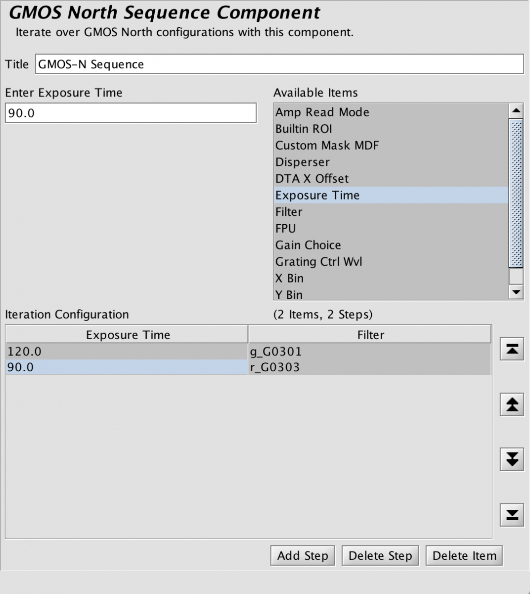
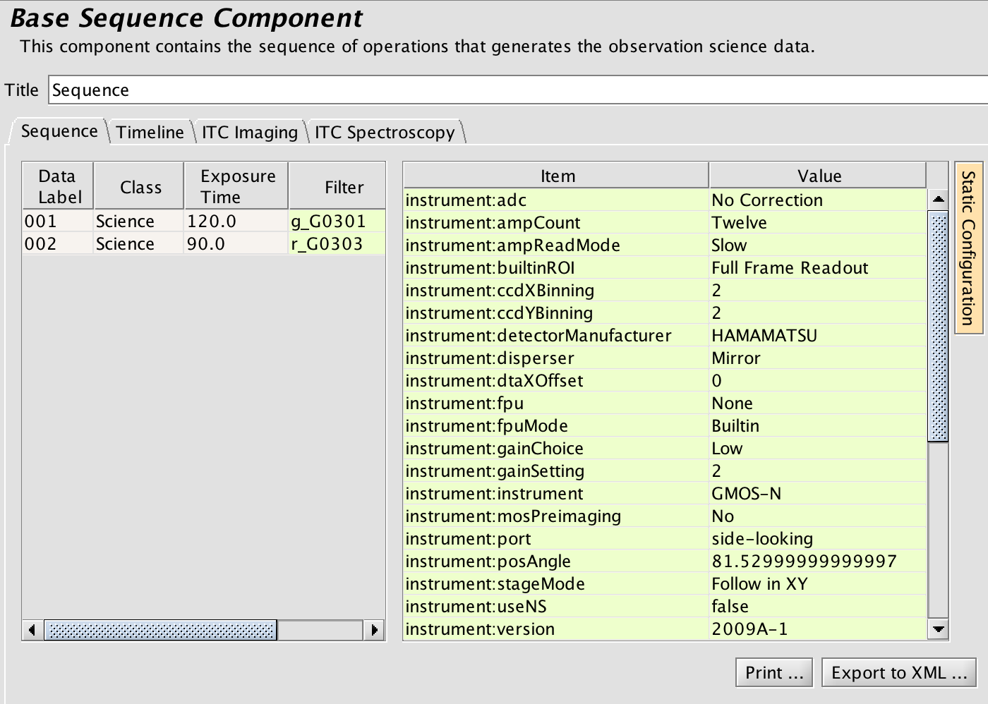
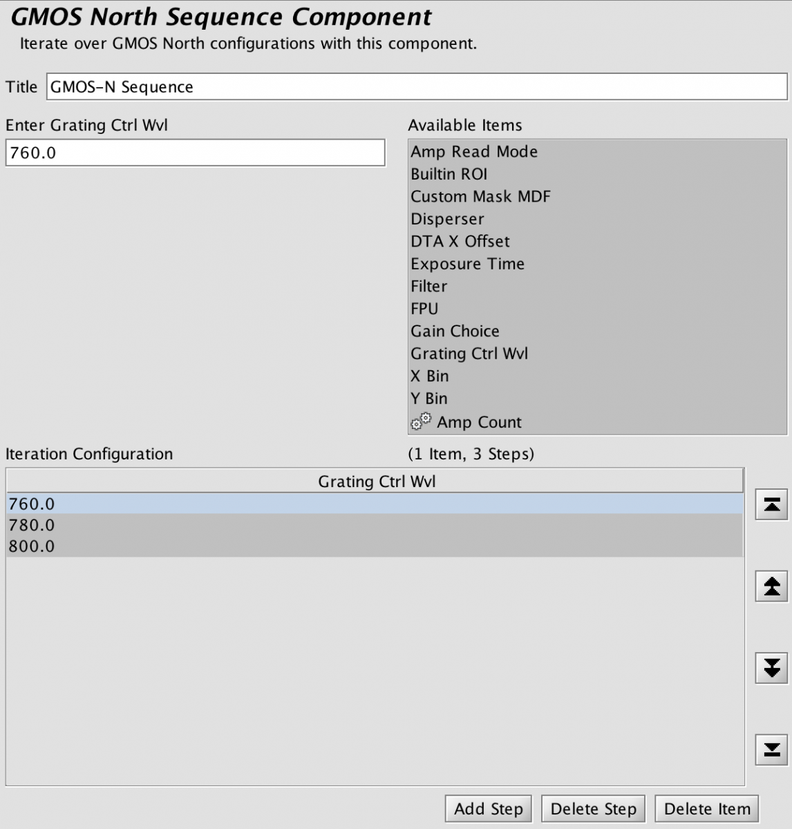
Example 2: GMOS Iterator longslit spectroscopy example
 |
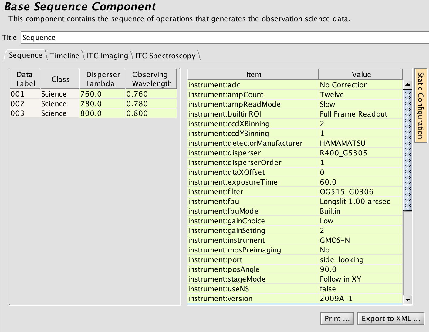 |
| GMOS iterator example for longslit spectroscopy | The resulting sequence with one observe element and no offset iterator |
In this example the sequence iterates over the central wavelength. Table rows correspond to iterator steps. At run time, all the values in a row are set at once. Since there are three steps in this table, an observe element nested inside the GMOS iterator would produce an observe command for each of three steps. Iteration of the central wavelength may be useful due to the gaps between the three detectors.
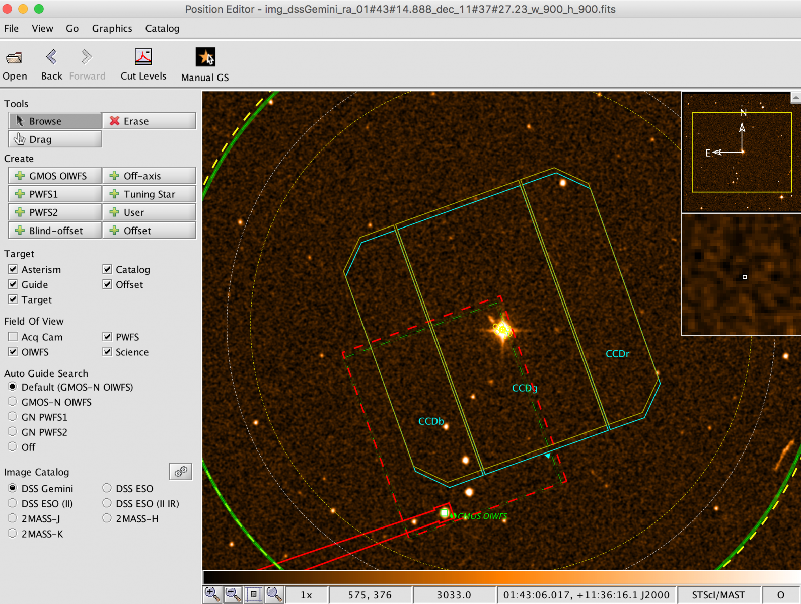
Viewing the GMOS On-Instrument Wavefront Sensor Field
GMOS is equipped with an on-instrument wavefront sensor (OIWFS). The region accessible to the OIWFS is a rectangular field, partly inside the imaging field of view, see the GMOS OIWFS page for details. The OIWFS arm vignettes a small part of the field of view if a guide star inside the imaging field of view is chosen. The vignetting and the region accessible to OIWFS can be viewed with the position editor by using the view...OIWFS FOV item in the position editor menu bar. An example of this is shown in the figure below; the accessible patrol field is outlined with the red dashed line and the projected vignetting of the OIWFS is shown shaded in red. If multiple offsets are defined the green dashed line delineates the region within which valid guide stars may be selected, showing the intersection of the accessible patrol field for all the offset positions. The example is shown for GMOS on the side-looking ISS port.
In cases where the science orientation is not critical, it is possible to rotate the instrument position angle to reach stars at other locations in the field.
OT Helpful Hint
This page contains useful information for configuring GMOS observations which should help reduce the number of iterations on the Phase II file between the PI and the NGO. It also contains an overview of the required OT observations and components for programs of different types. Before submitting your Phase II program to Gemini, use the GMOS Phase II checklist to eliminate common mistakes.
Contents
- GMOS Skeleton
- Required Observations and Components
- Overheads
- Imaging
- MOS
- Long-slit
- IFU
- Standard Stars
- Observations split over several nights
- Observing Conditions
Templates
A detailed description of all features related to the use of the Observing Tool (OT) template observations is provided on the OT help pages.
Required OT observations and components
For each type of program, there are different requirements to which OT observations and components the user has to define in the Phase II. The table below gives an overview over the requirements. "Required" means that a Phase II will not be accepted without this type of observation or component being defined. "As needed" means that the user can add this type of observation or component as needed by the science goals of the program. Use the GMOS OT library as a source of template and example observations.
CuAr arcs mixed with the science data, i.e. taken at night, and any special standard stars are charged towards the program's allocated time. Baseline standard stars, GCAL flats, twilight flats, baseline CuAr arcs, and mask images are not charged. The time for the acquisition observations is already included in the science observation overhead. No additional time is charged. However, the acquisition observations have to be defined as separate observations in the Phase II.
Each "Observe" is given a Class (see more details about Classes).
The details of each of the required observations and components are explained in the sections below.
|
Observation or Component |
Program Type | Class | |||
| Imaging (details) Pre-imaging for MOS |
MOS (details) | Longslit (details) | IFU (details) | ||
| Science Obs. | Required | Required | Required | Required | Science |
| Offset Comp. | As needed | As needed | As needed | As needed | N/A |
| GCAL flats | Do not add | Required Mix w/ science |
Required Mix w/ science |
Required Mix w/ science |
Nighttime Partner Calibration |
| Twilight flats | Do not add | As needed Separate observation |
As needed Separate observation |
Required Separate observation |
Daytime Calibration |
| CuAr arcs | N/A | Required Baseline: Separate observation |
Required Baseline: Separate observation |
Required Baseline: Separate observation |
Daytime Calibration |
| Charged if mixed w/ science | Charged if mixed w/ science | Charged if mixed w/ science | Nighttime Program Calibration |
||
| Acquisition Obs. | N/A | Required Separate observation |
Required Separate observation |
Required Separate observation |
Acquisition |
| If for baseline standard | If for baseline standard | If for baseline standard | Acquisition Calibration |
||
| Mask image | N/A | Required Separate observation |
N/A | N/A | Daytime Calibration |
| Baseline standard stars | Do not add | Required Separate observation |
Required Separate observation |
Required Separate observation |
Nighttime Partner Calibration |
| Nod & Shuffle Darks | N/A | As needed (for Nod & Shuffle only) Separate observation |
As needed (for Nod & Shuffle only) Separate observation |
As needed (for Nod & Shuffle only) Separate observation |
Daytime Calibration |
| Special standard stars Charged |
As needed Separate imaging observation |
As needed Separate longslit observation Follow requirements for longslit |
As needed Separate longslit observation Follow requirements for longslit |
As needed Separate IFU observation Follow requirements for IFU |
Nighttime Program Calibration |
Calculation of overheads
Detailed information about overheads for acquisitions (and reacquisitions), as well as readout and configuration times can be found on the GMOS overheads page. PIs can now use the calculated planned execution times in the OT as reasonable approximations of the actual time that will be required, with the exception that reacquisitions must be included when integrations times are long. If you do not take this into consideration, it is likely that your Phase II will be overfull. Gemini queue observers will stop executing your program when the allocated time has been depleted, regardless of whether or not there are still unexecuted observations.
If your observation classes are set correctly, the OT will not add any planned time for GCAL flats, twilight flats, baseline CuAr arcs or other daytime calibrations (eg mask images or Nod & Shuffle Darks). The support staff from your National Gemini Office and/or your Gemini Support Scientist will work with you if you have questions about your OT calculated program execution time.
Grating choices
All of the gratings included in the OT are available for science use. Only three of the gratings can be mounted in GMOS simultaneously. Grating changes will not be done during the night.
Program Organization
It is recommended that groups be used as much as possible to keep the Phase II organized. Some recommended organizational practices are:
- Group science observations with their associated acquisition observation(s).
- Organize all the time for long observations (more than 2 hours) into a single observation.
- If a standard observation must be taken before or after a science observation (e.g. a telluric standard) then place the observations for the standard in the same group as the science observations.
- Place all daytime calibrations in a folder called Baseline.
- Place time constraints (dates/times, temporal spacing of observations) within the new Scheduling Note and within the Timing Windows under Observing Constraints.
- Group names within a program should be unique.
Imaging observations
If full-frame readout is being used then an offset iterator should be used to define at least two offset positions separated by at least 10 arcseconds in p in order to fill in the chip gaps. The first offset position should always have p=0, q=0.
Twilight flats are baseline calibration and are handled by Gemini staff. Twilight or GCAL imaging flat observations should not be included in the Phase II.
Observations in the z'- or Y-bands are susceptible to fringing. Ideally, fringe frames can be derived from the science observations. If this is not possible or the baseline calibration (taken a few times per year) is not sufficient then blank sky observations need to be defined. The class should be 'Nighttime Program Calibration' and the time will be charged to the program. These observations should be like the science observations but the target component should be blank or removed. Gemini staff will add the appropriate blank sky field.
MOS observations
Programs that contain MOS observations require masks designed either from GMOS pre-imaging taken for all separate fields or from object catalogs. PIs with MOS programs are encouraged to submit designs as soon as possible, either early in the semester if designed from object catalogs or shortly after pre-imaging has been taken.
MOS programs should contain the final Phase II information for the pre-imaging observations when it is first submitted. The MOS observations should also be included in the program. Small adjustments to the MOS observations are allowed when the mask design has been done. However, the pointing and PA of your target cannot be changed between the pre-imaging and the MOS observations. PIs with MOS programs will be contacted by Gemini when the pre-imaging data is available. Revised Phase II MOS programs and mask designs should be submitted asap. See GMOS mask deadlines (linked from the relevant semester's OT instructions page) for Classical runs. Mask designs should be submitted directly through the OT, instructions will be sent to you when your pre-imaging is available.
PIs with pre-imaging from previous semesters should use the mask naming scheme (below) for their current program. Upload the original pre-imaging through the OT so that masks can be checked. Please also include a note listing the previous program number.
The focal plane unit for the MOS observations should be specified as Custom Mask MDF, and the field for the name should contain your program ID and a running number for the mask within the program, e.g. for program GN-2010B-Q-27 the mask names should be GN2010BQ027-01 and GN2010BQ027-02 for the first and the 2nd mask, respectively. Note the leading zero on the program ID and mask numbers.
The total time used for both pre-imaging and MOS observations must not exceed the allocated time.
It is recommended that pre-imaging observations are dithered by +/-5 arcsec in both directions, e.g. 4 exposures in a square pattern with size 5 arcsec will work ok. (Examples are available in the GMOS OT library). Pre-imaging exposures should be taken in the broad band filter closest to the central wavelength coverage of the MOS observations.
GCAL flats should be mixed with your science MOS observations. The baseline GCAL flats include one flat for each hour of open-shutter time, though a minimum of two flats is always taken. Make sure you get flats for all spectral configurations. GCAL flats within these guidelines have class 'Nighttime Partner Calibration' and are not charged to the program. Any additional GCAL flats should have class 'Nighttime Program Calibration' and will be charged to the program. The smartGCAL flats will automatically determine the best exposure times for the instrument configuration.
CuAr arcs taken during the day are baseline calibrations. These calibrations are not charged to the program, but the PI has to define them in the Phase II. Define these observations as separate from the science observations and set the class to 'Daytime Calibration'. Make sure the instrument configuration matches the science observation. If you copy the science observation in order to edit it for the CuAr arc, make sure to remove the guide star from the target component, remove any science exposures, and change the class. Arcs taken as part of a science MOS observations should have class 'Nighttime Program Calibration' and will be charged to the program. The smartGCAL arcs will automatically determine the best exposure times for the instrument configuration.
Mask images are taken of all MOS masks before they are used for science. These calibrations are not charged to the program, but the PI has to define them in the Phase II. Define these observations as separate from the science observations. By applying the OT templates, a mask image observation is automatically created for each target. For a complete example see the GMOS OT Library.
Acquisition observations need to be defined for each MOS mask. No extra time is charged for these observations, as the overhead for setting up is already included in the science observation. However, the acquisition observations should be defined as separate observations in the Phase II. By applying the OT templates, an acquisition observation is automatically created for each target. The acquisition observation needs to have the same target, guide star, and PA as the science observation. Make sure that the exposure time (typically 30-90 sec) and filter match the setup required for the mask acquisition stars. Long-pass filters cannot be used for MOS acquisitions. Narrow band filters should in general not be used for MOS acquisitions.
The acquisition template "MOS: Acq starting with the mask in the beam" should only be used if the MOS mask was designed from pre-imaging obtained with the same GMOS instrument and using the same CCDs. MOS masks designed from other data (catalogs, pre-imaging using the previous GMOS CCDs, etc.) will need to be acquired using the "MOS: Acq starting with the mask out of the beam" template. The support staff from your National Gemini Office and/or your Gemini Support Scientist can provide further details regarding the use of the two different templates. See also the example in the GMOS OT Library.
Twilight flatfields are taken for each MOS mask if requested. No extra time is charged for these observations. However, the twilight flatfields should be defined as separate observations in the Phase II. Make sure the instrument configuration matches the science observation. If you copy the science observation in order to edit it for the twilight flatfield, make sure to remove the guide star from the target component, then edit the science exposures to have only one exposure with 30sec exposure time. The class should be 'Daytime Calibration.' If doing small wavelength dithers to fill in the chip gaps then only one wavelength setting will have a twilight flatfield taken, so you need to select the wavelength at which you want the twilight flatfield. If there are no twilight flats in the submitted Phase II for a MOS program, it will be assumed that they are not needed. See also the example in the GMOS OT Library.
Long-slit observations
GCAL flats should be mixed with your science observations. The baseline GCAL flats include one flat for each hour of open-shutter time, though a minimum of two flats is always taken. Make sure you get flats for all spectral configurations. GCAL flats within these guidelines have class 'Nighttime Partner Calibration' and are not charged to the program. Any additional GCAL flats should have class 'Nighttime Program Calibration' and will be charged to the program. The smartGCAL flats will automatically determine the best exposure times for the instrument configuration.
CuAr arcs taken during the day as baseline calibrations. These calibrations are not charged to the program, but the PI has to define them in the Phase II. Define these observations as separate from the science observations and set the class to 'Daytime Calibration'. Make sure the instrument configuration matches the science observation. If you copy the science observation in order to edit it for the CuAr arc, make sure to remove the guide star from the target component, remove any science exposures, and change the class. Arcs taken as part of a science longslit observation should have class 'Nighttime Program Calibration' and will be charged to the program. The smartGCAL arcs will automatically determine the best exposure times for the instrument configuration.
Acquisition observations need to be defined for each longslit target. No extra time is charged for these observations, as the overhead for setting up is already included in the science observation. However, the acquisition observations should be defined as separate observations in the Phase II. For Point Sources a ROI of Central Stamp (300x300 unbinned pixels) should be used to measure the slit center and to confirm if the science target is within the slit. For Extended Objects, Double Sources and Off-axis Sources a ROI of CCD2 should be used to measure the slit center and confirm if the object is within the slit. By applying the OT templates, an acquisition observation for each target will be automatically created. The acquisition observation needs to have the same target, guide star, and PA as the science observation. Make sure that the exposure time and filter match the setup required for the target. Long-pass filters cannot be used for longslit acquisitions. Narrow band filters should only be used if your target is an emission line source with no continuum. For a complete example see GMOS OT Library.
Twilight flatfields Twilight flats, which provide information about the slit function, are usually not taken for longslit programs, but can be provided if requested. No extra time is charged for these observations. However, the twilight flatfields should be defined as separate observations in the Phase II. Make sure the instrument configuration matches the science observation. If you copy the science observation in order to edit it for the twilight flatfield, make sure to remove the guide star from the target component, then edit the science exposures to have only one exposure with 30sec exposure time and class 'Daytime Calibration'. If doing small wavelength dithers to fill in the chip gaps then only one wavelength setting will have a twilight flatfield taken, so you need to select the wavelength at which you want the twilight flatfield. See also the example in the GMOS OT Library. If there are no twilight flats in the submitted Phase II for a longslit programs, it will be assumed that they are not needed.
IFU observations
IFU observations can be done either in "two-slit mode" or "one-slit mode". For GMOS observations in "one-slit mode" the "IFU Right slit (red)" must be chosen. (The Blue slit is not offered due to a larger number of broken fibers). The change between the two modes is a manual process that involves taking the IFU out of the instrument. This will not be done during the night. GMOS is used for blocks of time in either mode, and changes between the modes are done infrequently.
The OT visualization of the GMOS IFU shows the larger of the two IFU fields at the target position. Thus, if switching between fpu=none and the IFU, the user will see the OIWFS field patrol field move -- this is as expected, since the larger of the two IFU fields is approximately 30 arcsec from the center of the imaging field of view.
In one-slit mode the central wavelength you specify will be interpreted as the desired wavelength at the center of the detector array. In two-slit mode, the central wavelength you specify will be the wavelength at the location of the two pseudo-slits.
In two-slit mode you will have to use one of the color filters in order to avoid overlap between the spectra, see the grating/filter combinations page for details. In 1-slit mode you may have to use a filter to avoid 2nd order contamination.
GCAL flats should be mixed with your science observations. For IFU observations it is particularly important to take GCALflats frequently as flexure can impact the fiber tracing. The baseline GCAL flats include one flat for each hour of open-shutter time, though a minimum of two flats is always taken. Make sure you get flats for all spectral configurations. GCAL flats within these guidelines have class 'Nighttime Partner Calibration' and are not charged to the program. Any additional GCAL flats should have class 'Nighttime Program Calibration' and will be charged to the program. The smartGCAL flats will automatically determine the best exposure times for the instrument configuration.
CuAr arcs taken during the day as baseline calibrations. These calibrations are not charged to the program, but the PI has to define them in the Phase II. Define these observations as separate from the science observations and set the class to 'Daytime Calibration'. Make sure the instrument configuration matches the science observation. If you copy the science observation in order to edit it for the CuAr arc, make sure to remove the guide star from the target component, remove any science exposures, and change the class. Arcs taken as part of of a science IFU observation should have class 'Nighttime Program Calibration' and will be charged to the program. As flexure can have a noticeable impact on IFU observations, it is recommended to include arcs in the science IFU observation, especially if the wavelength coverage does not include any sky lines. The smartGCAL arcs will automatically determine the best exposure times for the instrument configuration.
Acquisition observations need to be defined for each IFU target. No extra time is charged for these observations, as the overhead for setting up is already included in the science observation. However, the acquisition observations should be defined as separate observations in the Phase II. By applying the OT templates, an acquisition observation for each target will be automatically created. The acquisition observation needs to have the same target, guide star, and PA as the science observation. Make sure that the exposure time (typically 2-5 min.) and filter match the setup required for the target. Longpass filters cannot be used for IFU acquisitions. Narrow band filters should only be used if your target is an emission line source with no continuum. See also the example in the GMOS OT Library.
Twilight flatfields are taken for IFU observations. No extra time is charged for these observations. However, the twilight flatfields should be defined as separate observations in the Phase II. Make sure the instrument configuration matches the science observation. If you copy the science observation in order to edit it for the twilight flatfield, make sure to remove the guide star from the target component, then edit the science exposures to have only one exposure with 90sec exposure time with class 'Daytime Calibration'. For small spectral dithers, twilight flats are typically only taken for one wavelength setting. See also the example in the GMOS OT Library.
Standard Stars
Imaging standards sufficient to obtain flux calibration at the 5% level are base calibrations and are taken by Gemini staff. If better calibration is needed then observations for additional standards must be included in the Phase II. The class should be 'Nighttime Program Calibration' and the time will be charged to the program.
Spectroscopic flux standards sufficient to determine the spectral response function, not absolute flux calibration, are baseline calibration and are not charged to the program. Observations for the baseline flux standard need to be defined in the Phase II. All MOS flux standards are taken in longslit mode (using the longslit closest in width to the width of the MOS slitlets in MOS mode). All standard star observations should have the observing conditions set to 'Any' and should have the target component deleted and the PA set to 'average parallactic'. The observer will fill in the target and align the PA to the parallactic angle when taking the standard. Baseline standard observations consist of the following components:
- Acquisition with class 'Acquisition Calibration': The longslit acquisition sequence for all standard stars (flux standard, velocity standards, etc) uses an ROI of Central Stamp (300x300 unbinned pixels) to image the field, measure the slit center, and to confirm if the target is within the slit. (For GMOS-N, the IFU acquisition sequence for standard stars includes a ROI of Central Stamp to image the field. For an IFU acquisition, the offsets from the center of the CCD2 to the IFU-1 and IFU-2 fields are well known by the telescope observers and do not need to be defined.) See the examples included in the GMOS OT Library.
-
Spectroscopic observation with class 'Nighttime Partner Calibration': Please select an exposure time long enough to obtain good signal-to-noise (i.e., 120 seconds). The instrument configuration should match the science observations (using the longslit closest in width to the width of the MOS slitlets in MOS mode). For longslit and MOS programs, the spectroscopic observations should have the ROI defined as central spectrum. For MOS mode, if the grating is not the R150, then a GMOS sequence should be used to define three wavelength settings that will bracket the expected wavelengths of the MOS observations. The three recommended wavelength settings for each grating are shown in the table below. GCAL flats at each wavelength setting should be included. Examples can be found in the GMOS OT Library.
-
Daytime arcs with class 'Daytime Calibration'. All wavelength settings used by the nighttime observation should be included. All other guidelines for daytime arcs apply.
| Grating | First Setting | Second Setting | Third Setting |
| R400 | central wavelength - 150 nm | central wavelength | central wavelength + 150 nm |
| B/R600 | central wavelength - 100 nm | central wavelength | central wavelength + 100 nm |
| R831 | central wavelength - 80 nm | central wavelength | central wavelength + 80 nm |
| B1200 | central wavelength - 30 nm | central wavelength | central wavelength + 30 nm |
Recommended wavelength settings for standard star observations obtained for MOS programs
Additional spectroscopic standards --- absolute flux standards, velocity standards, line-strength standards, telluric standards, etc.--- must also be defined. If absolute flux calibration is desired then the 5arcsec-wide longslit should be used and at least three wavelength settings should be used, as in the MOS spectral response calibration above, to cover the full wavelength ranges of most gratings. Recommended settings are the same as the ones given in the table above.
The guidelines are the same as for normal longslit observations except that the classes for the on-sky observes should be 'Nighttime Program Calibration' and the time will be charged to the program. The associated acquisition observations should have class 'Acquisition' and any GCAL flats are still 'Nighttime Partner Calibration'. Daytime arcs are always 'Daytime Calibration' and are not charged.
Observations that will be split over several nights
Some observations cannot be completed within one night and therefore will require multiple acquisitions. Exactly how such an observation will be split in several observations over several nights will normally be determined by the Gemini Staff at the time of scheduling the night's observations (see the overheads page for guidelines). The user should define such observations as one observation, and add a comment to explain which assumptions were made about the number of reacquisitions and the resulting overheads.
Observing conditions
The observing conditions are specified as percentiles in image quality, cloud cover, sky background (and water vapor). Refer to the observing conditions page for details about the meaning of these percentiles. If the percentiles do not give sufficient information to the queue observer about the observing conditions required for a given observation, the user should add a comment to the observation detailing the observing conditions, e.g. "Need fwhm better than 0.75 arcsec in r". Such comments cannot be used to request better observing conditions than approved by the time allocation process.
Baseline calibrations
GMOS Baseline calibrations that are not specifically mentioned above should not be included in the Phase II programs prepared by the users.
Phase II Checklist
Checklist for GMOS Phase II (OT) programs
- General
- Have you selected appropriate templates from the GMOS OT library? Have you gone through the checklist in the Top-level Program Overview note and included relevant standardized notes? Add notes with information about the program and acquisition that will make it easier for the observer. Try to use the standardized notes provided in the OT Library.
- In the GMOS component, check that readout, translation stage, and ROI are correctly defined for the observation type. If in doubt, see the relevant examples in the GMOS OT library. Make sure that nighttime science observations have the Translation Stage set to Follow and daytime calibrations set to "Do Not Follow" or "Follow in Z Only" (GMOS-S). Check also that the Region of Interest that will be read out is appropriate for the observation type and that the read mode is set to Fast Read/Low Gain for acquisitions, daytime calibrations etc, and to Slow Read/Low Gain for science observations (or Fast Read/High Gain for bright targets). The CCD readout must be set to Use 12 amplifiers for the Hamamatsu GMOS-N and GMOS-S CCDs.
- Is the binning set appropriately for the instrument configuration and requested observing conditions? Basically, make sure your are optimizing the pixel sampling of the spatial resolution (GN/GS) and/or the spectral resolution.
- Are the integration times reasonable? Individual imaging observations should not be longer than 10-15min, individual spectroscopy observations should not be longer than 20min (GMOS-S and GMOS-N Hamamatsu CCDs, due to the high rate of cosmic rays). Short exposures result in large overheads from the readout of the detectors, and may give data dominated by the read-noise.
- GMOS observation sequences that take longer than ~2 hours to execute will likely not be executed all on one night, and you must allow adequate time for re-acquisitions on subsequent nights when filling the allocated time. Have you read the details about the overhead calculations? Have you added a note explaining how many reacquisitions you have assumed for the calculation of the overheads? Taking the correct overheads into account, do your defined observations fit within the allocated observing time? Is there an appropriate mix of science exposures and baseline calibrations in the sequence? Spectral flats at redder wavelengths should be taken about once per hour, while flats at bluer wavelengths can be taken in the daytime.
- Have you checked Baseline Calibrations to see what is offered/required.
- Baseline arcs and flats should be set up using smartcals now. Choosing a flat (as observe element) within a science sequence will automatically set up a baseline nighttime partner calibration with an optimal exposure time. Choosing an arc within a science sequence will automatically set up the correct exposure time but these must be set to nighttime program calibration. Within a daytime arc sequence, this will be set up as daytime partner calibration. If you feel you need a different exposure time (e.g., because the desired grating/filter/wavelength/slit width combo is not known by the smart cal library), please contact your Gemini program Contact Scientist, or file a helpdesk ticket. As of 2012B, arcs and flats configured manually will no longer be checked by either the NGO or Contact Scientist. Any time lost will be charged to the PI.
- Have all observation classes been set correctly?
- Have you considered the effects of differential atmospheric refraction on your data? The default position angle has been set to 90deg in the GMOS-N and GMOS-S Libraries, as for most science targets this will minimize the slit losses. However, if your target Declination differs from the observatory latitude by more than ~ 25-30 deg (for targets observed with GMOS-N Dec > +50 or Dec < -10, for targets observed with GMOS-S Dec > 0 or Dec < -60), at a minimum the position angle should be changed to 0 deg if possible. More information is available on why target Dec influences the choice of default position angle. If desired, take longslit observations at the parallactic angle. To do so, please include a note with the title OBSERVE AT MEAN PARALLACTIC ANGLE in the program. If this is not possible, the hour angle/airmass constraints can be chosen to ensure that the target is observed closer to transit. These will need to be approved by the appropriate Head of Science Operations.
- Guide stars
- Are guide stars selected for the GMOS OIWFS? The PWFSs are not used for observing sidereal targets with GMOS in most cases. First, select the position angle mode (Fixed, Allow 180deg flip, Average parallactic) in the GMOS component as appropriate. The automatic guide star selection service will select an appropriate guide star for the specified observing conditions. Alternatively, the PI can still choose a guide star using the Manual GS button on the OT position editor. For manual guide stars, ensure that the guide star can be reached for the selected position angle, that the guide star is within the magnitude limits for the OIWFS, and that all guided offset positions can be reached. Check that the probe arm is visible and falls within the green box in the position editor. Fix any red offset positions. The UCAC4 catalog should be used whenever possible for choosing guide stars as the magnitudes are usually reliable.
- Ensure guide stars are stars and not galaxies.
- Calibrations
- Check that appropriate calibrations are included in the program. To see which baseline calibrations/standards are recommended, see Baseline Calibrations.
- For baseline spectrophotometric standards or twilight flats, make sure that the target component is left blank or excluded.
- If the PI requires calibrating standards beyond what is offered in the standard baseline calibrations, these must be defined, including a specific target, and time will be charged against the program for the observation. Observing class should be set to Nighttime Program Calibration. Baseline standards are set to partner calibration.
- Imaging
- Note that binning is recommended for imaging observations in IQ70 conditions or worse.
- Have you considered spatial dithers for imaging? There are gaps between the three detectors in GMOS, illustrated on the GMOS imaging page and whose approximate positions are indicated in the OT position editor.
- If imaging in the i, z, Z, and Y-filters, have you considered how to handle the fringing? In GMOS-N and GMOS-S the fringing becomes apparent redward of about ~800 nm and is about ~2% of the background level in the Y-band (GMOS-N and GMOS-S), and ~1% (GMOS-N)/less than 0.5% (GMOS-S) in the z'-band. A minimum of 5 exposures is recommended in order to generate a good fringe frame.
- Baseline photometric standards should not be defined within the program. These baseline standards are already taken on each photometric night that imaging data is obtained. If the PI wishes to have more than one taken, or insists on having one taken with a program defined for CC70 conditions, then a program standard with target component will have to be defined in the program by the PI.
- Spectroscopy
- Have you considered spectral dithers for spectroscopy? There are gaps between the three detectors in GMOS, illustrated on the GMOS long-slit spectroscopy page. If complete wavelength coverage is essential, then two sets of observations with slightly different wavelengths are needed. The recommended minimum shifts are ~20nm for the R150 grating, ~7.5nm for the R400 grating, and ~5nm for all other gratings. Please also note the updated recommendations on dither strategies to deal with the GMOS-N and GMOS-S detector artifacts.
- At long wavelengths, fringing becomes a problem. If not using N&S to correct for the sky background, it is best to use spatial dithers from which fringe frames can be generated.
- Ensure that all the appropriate baseline calibrations (nighttime GCAL flats, twilight flats, daytime CuAr, mask image obs [for MOS], and spectrophotometric [flux response] standards) and acquisition observations are included.
- Have you considered including nighttime calibration arc lamp exposures in the science sequences? Due to flexure in the instrument, nighttime arc lamp exposures for blue spectroscopic setups which do not cover at least the 5577 A sky line are included as part of the Baseline Calibrations (see Baseline Calibrations for details about the specific grating and central wavelength configurations for which on-sky arcs are provided). On-sky arc calibrations for other setups, if required, can be requested as part of the program time.
- For spectroscopy at wavelengths longer than about 850 nm, the wavelength calibration can be improved by including 2nd-order CuAr lines in the wavelength calibration. In this case, it may be beneficial to take additional CuAr exposures without any order-blocking filter. An example line list can be found here.
- Have you included the appropriate acquisition observations?
- If an observation includes an unusual or non-standard acquisition (eg. off-axis long-slit or IFU where the guide star cannot be accessed with the science target on-axis, blind offset acquisitions, MOS acquisitions with large initial offsets, etc), include the appropriate OT Library standardized note in the program. The text of the note can either describe the acquisition or point to other notes within the program. Using these standardized notes should minimize acquisition errors and observers won't be surprised. See the OT library for examples of non-standard acquisitions. See COMPLETE EXAMPLE: Longslit (extended/double/off-axis source), for cases where the science object is either extended by more than 15", a double source where the targets are separated by more than 20", or a target which is more than 20" off-axis in the q-direction.
- BLIND OFFSETS: Use when targets are too faint to be acquired within 1 min of direct imaging.
- Make sure that a Blind-offset (1) target is defined with coordinates on the same astrometric system as the science.
- Make sure the Blind-offset (1) star has a name.
- Offset star should preferably be within 20 arcsec of the science target. The accuracy of blind offsetting is better than 0.1 arcsec for offsets less than 20 arcsec.
- For the blind offsetting to work, it is essential that the same guide star can be reached for the bright object and the science target.
- Include a note in the program to warn the observer of the non-standard acquisition.
- If your longslit or IFU spectroscopic observations involve complicated alignments, crowded fields, or targets fainter than about R=18 (eg. if the target is not obvious in the OT position editor with the Digitized sky survey 2 image loaded), you need to prepare finding charts. Such a finding chart should indicate the target/s and display the orientation (preferably North up and East to the left) and scale. Finding charts should be uploaded through the OT.
- Have you included the observation for the flux (spectral-response) standard? For MOS, standard star observations should be taken at 2-3 central wavelengths in order to span the full wavelength range over the mask (see the Description in the MOS Baseline Calibration Examples in the OT LIbrary). Otherwise, if spectral dithers are used in the science, only one central wavelength will be observed for the flux standard. Do not include a target component (or if included, please leave the target blank) for baseline standards. The observer will choose one appropriate for the time of the observation.
- Have you considered using Nod&Shuffle for spectroscopy in the red?
- If using N&S, check that electronic offsetting is chosen if small offsets (< 2.0arcsec) have been defined (this will reduce overheads significantly).
- Recommended exposure times are 60s for CC50/70 and 30s for more variable and thick cloud conditions.
- The nod should be less than half the length of the slit if the observation intention is to keep the object within the slit for both nods. For large nods, if the guide star cannot be reached at the sky position, make sure the OIWFS is set to freeze.
- Ensure that the shuffle distance defined in the Nod & Shuffle tab makes sense. For microshuffling, the distance should be the same as the slit length (but must be an even number of rows if binning by 2).
- Check that a N&S dark is defined in order to correct for charge traps. For deep observations it is also recommended to translate the detector a few pixels in the y-direction between N&S observations. Check that the observations have been split into multiple dithered exposures, with the translation of the detector set by the DTA-X offset. For the GMOS-S and GMOS-N Hamamatsu detectors, charge traps are not present. Therefore N&S darks and DTA-X offsets are no longer necessary, but if these are defined the minimum allowed value for DTA-X offset is -2. (The maximum DTA-X offsets for GMOS-N are +/-4.)
- For IFU observations, make sure that the guide star can be reached in both the acquisition and science observation. If it is not possible, choose a guide star appropriate for the science observation and include a standardized note in the program warning of this.
- Binning: check that the Y-direction is left unbinned since the width of each IFU fiber is only 5 unbinned pixels. Since the spectral resolution in the IFU is equivalent to 4.26 unbinned pixels, binning in the spectral direction for very faint objects may be useful.
- If you are using the IFU in two-slit mode, you will have to use one of the color filters to avoid overlap between the spectra. For IFU observations in one-slit mode, IFU-R should be chosen over IFU-B (IFU-R is recommended over IFU-B for both GMOS-N and S).
- If your program is a MOS program, have you defined any pre-imaging along with mask observations? You will get the chance to modify the MOS observations once you design your mask. However, the pointing and PA of your target cannot be changed between the pre-imaging and the MOS observations.
- If taking pre-imaging, make sure the MOS pre-imaging option on the OT GMOS component is indicated.
- If no pre-imaging was taken, make sure the acquisition starts with a mask out of the beam step for coarse alignment.
- For MOS programs, have you included the required daytime calibration mask image(s) .
- If your program is a MOS program, prepare yourself for the mask design by reading the MOS instructions in detail and installing the required software.
- Mask names must be in the correct format: ie for program GN-2003B-Q-27, the mask names should be GN2003BQ027-01 and GN2003BQ027-02 for the first and second mask, respectively.
- If a mask was designed from a catalog, make sure the RA, Dec, and position angle entered in the OT are the same values used for making the mask. You can extract the RA and Dec information from the MDF file or pseudo image (eg by using "thselect {maskfile.fits} RA_IMAG,DEC_IMAG" or "hselect {psuedo_image} RA,DEC in pyraf). Check the PA by comparing the pseudo image orientation (after inverting y and rotating to the PA listed in the OT) with eg. a DSS image in the OT position editor.