Announcements
This section focuses on how to prepare NIRI observations for your Phase I and Phase II submissions. Preparing observing sequences involves much more than setting up the observation of the target; the complete observing sequences must include in addition "acquisition observations" (e.g., for finding the target and centering it on the image ) if needed, observations of telluric standards and/or flux standards, and usually includes flat field calibrations and dark frames.
The key to successful observation preparation is starting from the NIRI Observing Tool (OT) Library when creating your Phase II in the OT. An additional description of required supporting observations for NIRI is given on the Near-IR Resources page.
Below are some useful links to help you get started with your Phase I with the PIT (Phase I Tool) and Phase II preparation with the OT
Overheads
Acquisition overheads associated with setting up on each new science target include time for slewing the telescope, configuring the instrument and WFS, and in the case of (archival) spectroscopic observations, centering the target in a slit.
Long imaging observations may be split over several nights to better accommodate them in the queue. Please allow for one acquisition for every 1.5 - 2 hours of observing when calculating the time required for your project.
In imaging mode automated dither patterns have an estimated on-source efficiency of ~75%, where 25% of the elapsed time is used for telescope offsetting, WFS re-acquisition, detector readout etc; the exact overheads vary with the size of the offset and the exposure time.
All of the values listed on this page are included in OT calculations of the execution time of an observation. However, only the actual overheads incurred at the time of the observation will be charged to the program.
Table 1: NIRI acquisition overheads.
| Action | NIRI + PWFS | NIRI + Altair NGS | NIRI + Altair LGS |
| Imaging Acquisition | 6 min | 10 min | 15 min |
Table 2: NIRI overheads for each image.
| Array Size | Low Background | Medium Background | High Background |
| 1024 x 1024 | 5.0s + 11.16s * Ncoadds | 5.09s + 0.71s * Ncoadds | 5.11s + 0.20s * Ncoadds |
| 768 x 768 | 5.12s + 6.48s * Ncoadds | 5.14s + 0.41s * Ncoadds | 5.14s + 0.11s * Ncoadds |
| 512 x 512 | 5.11s + 3.10s * Ncoadds | 4.99s + 0.21s * Ncoadds | 5.12s + 0.08s * Ncoadds |
| 256 x 256 | 5.12s + 0.98s * Ncoadds | 5.17s + 0.08s * Ncoadds | 5.17s + 0.04s * Ncoadds |
Table 2 gives estimates of the overheads associated with taking NIRI images in the various array geometries and read modes without telescope offsetting. These values include the time to read out the array Ncoadds times and to write the final FITS image. The overhead for telescope offsetting depends on the distance of the offset, but is typically ~5 seconds for small offsets.
OT Details
The instrument non-specific aspects of the Observing Tool (OT) are described elsewhere. Detailed information on NIRI Component of the OT and the NIRI Iterator is provided below.
The detailed component editor for NIRI is accessed in the usual manner, by selecting the NIRI component in the science program, and is shown below:
Selecting a camera, etc.
Choice of camera, beam splitter, filter, dispersing element and focal plane mask (slit) is made by clicking on the pull down lists (i.e. the down-pointing arrows) and selecting the desired item. For example, there are three cameras f/32, f/14 and f/6, which are normally used with the "same as camera" slitter or f/6 beam splitter. Note how the window displaying the science field of view changes automatically to reflect the choice of camera, focal plane mask, and beam splitter. For direct imaging no dispersing element is required.
If you display a view of the field with the position editor and have selected the "science area" button, then this too will reflect the choices of NIRI camera and focal plane mask.
Selecting a filter
For imaging observations, the filter is chosen by selecting one from the list (by clicking on it). The central wavelength is given for each filter to assist with identification. You can move the vertical slider bar or click on the arrow buttons to browse the list. Note that the proper order-sorting filter should be selected for grism spectroscopic observations.
Controlling the exposure
The exposure time is set by clicking in the relevant window and typing the required number of seconds. Each occurrence of the observe element will cause N exposures to be taken and coadded in the instrument control system. The value of N is set by typing an integer in the "coadds" window. The total exposure in each output image will be the exposure times the number of coadds.
The total exposure time (single exposure x coadds x nods) in a single observation should not exceed 4 hours for imaging.
Setting the position angle
The facility Cassegrain Rotator can rotate the instrument to any desired angle. The angle (in conventional astronomical notation of degrees east of north) is set by typing in the "position angle" window. The view of the science field in the position editor will reflect the selected angle. Alternatively the angle may be set or adjusted in the position editor itself by interactively rotating the science field.
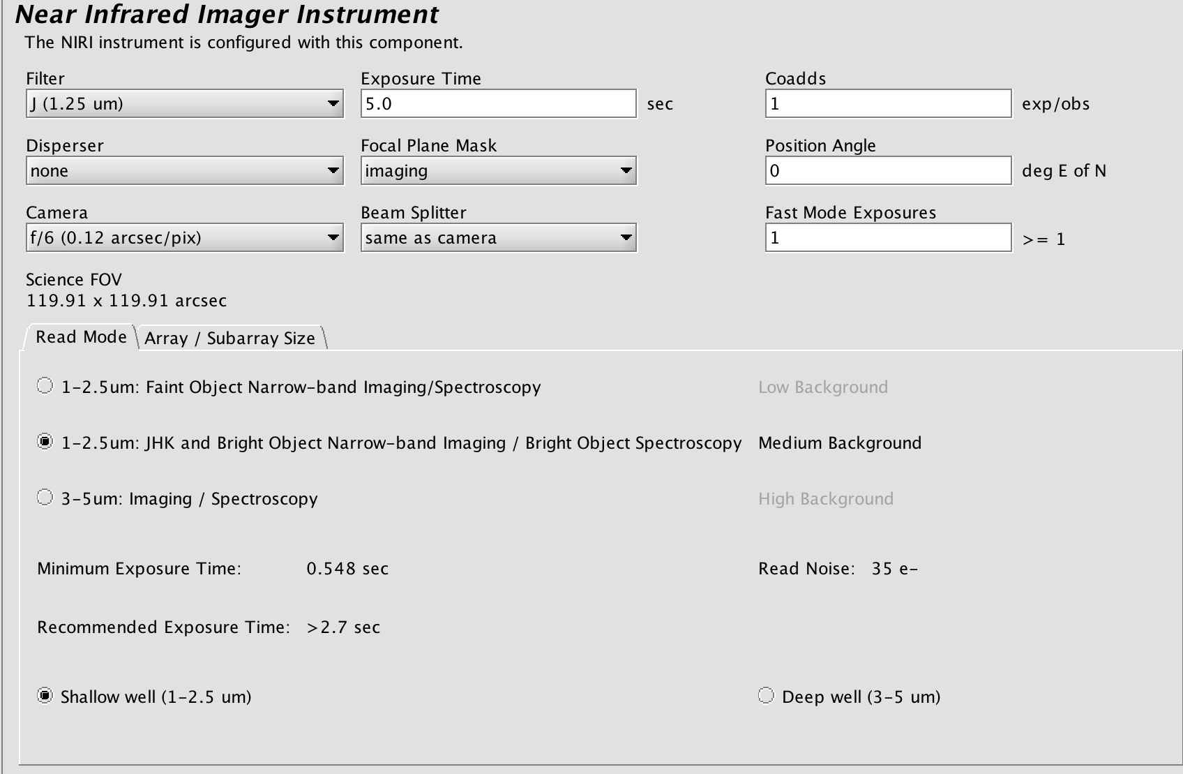
Array readout mode
The NIRI array is read out in different modes for different kinds of observations. Select the button corresponding to the desired mode. Note that the read noise, recommended minimum exposure time, and suggested background regime are indicated in green to the left and below; they change as the different read modes are selected. The array bias voltage can also be set for "deep well" and "shallow well." The choice of bias voltage affects the well depth, but not the minimum integration time or read noise. Note that the array read mode can be changed in the NIRI iterator, but the bias voltage cannot.
Regions of interest
A smaller sub-array can be read out more quickly than the whole NIRI array. By clicking on the "Regions of Interest" tab, one sees the options available: full frame readout (1024x1024 pixels), central 768x768, central 512x512, or central 256x256. As implied by their description, each subarray is centered on the detector. The sub-array readout should be used to reduce the minimum integration time. Note that the subarray size can be changed in the NIRI iterator by selecting "Builtin ROI" from the Available Items.
Saving changes
Any changes made in the OT are stored locally. These do not get sent to the Gemini online database unless the program is synced. The sync button (on the top right of the OT) accepts the latest changes and stores the newly updated program to the Gemiini database. You can also export your program locally to an XML file through File-->Export as XML which can be later imported back into the OT if needed.
NIRI Iterator
The NIRI Iterator is a member of a class of instrument iterators. Each works exactly the same way, except that different options are presented depending upon the instrument. Below we see a few of its features:
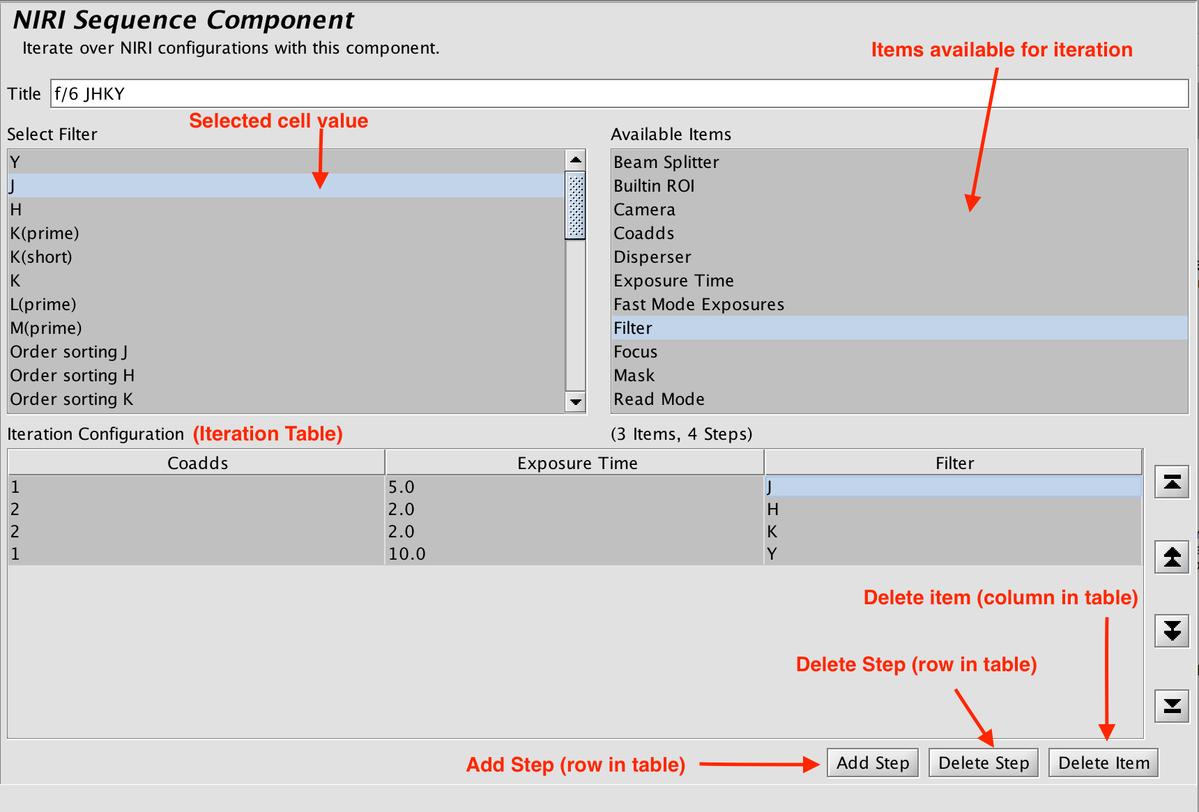
An iteration sequence is set up by building an Iteration Table. The table columns are items over which to iterate. In this example, the program is iterating over filters and exposure time so there are two corresponding columns in the table. Table rows correspond to iterator steps. At run time, all the values in a row are set at once. Since there are three steps in this table, an observe element nested inside the NIRI iterator would produce an observe command for each of three filters, using the specified integration times:
The items that are available for inclusion in the iterator table are shown in the box in the upper right-hand corner. Selecting one of these items moves it into the table in its own column. Each cell of the table is selectable. The selected cell is highlighted green. When a cell is selected, the available options for its value are displayed in the box in the upper left-hand corner. For example, when a cell in the filter column is selected, the available filters are entered into the text box. When a cell in the integration time column is picked, the upper left-hand corner displays a text box so that the number of seconds can be entered.
Rows or columns may be added and removed at will. Rows (iteration steps) may be rearranged using the arrow buttons.
Phase II (OT) Checklist
- Have you completed the General Gemini Phase II checklist?
- Guider:
- When using PWFS2 the guide star must not be too close to the center or the probe arm may vignette the detector on some of the offset positions. This may be acceptable if the target is small or off-center, but it should be avoided if possible.
- When using PWFS2 the guide star must not be too close to the edge or it may be unreachable in some offset positions. This can be checked by using the Position Editor to visualize the probe positions for each offset step.
- The guide state in the offset iterator should be "guide" for all science dithers, and typically "freeze" for the sky dithers. Sky dithers can be guided if they are close enough to reach with the same guide star and if not offsetting frequently, as the guide probe moves rather slowly and therefore waiting for the guider will incur extra overhead
- OT Setup:
- Acquisitions are typically not necessary for f/6 imaging as the field of view is quite large (120"). Acquisitions are recommended to get the best centering on f/32 imaging.
- The sky background (which refers to optical sky background) should be set to "Any" for almost all near-IR (1-5 microns) observations.
- The water vapor should be set to "Any" for 1-3 micron observations and carefully considered for observations at wavelengths >3 microns.
- An extra offset is recommended to compensate for the first frame effect. This extra offset may be at the beginning (historically called a "dummy" frame) or simply added at the end.
- If there is a chance that any source will saturate the PI should include a note telling the observer what to do. Possible actions include: 1) nothing, 2) stop the observation and request feedback from the PI, 3) decrease the exposure time, 4) decrease the exposure time and increase the number of coadds. Decreasing the exposure time may require changing the read mode and/or array ROI, so the note should state whether these changes are allowed.
- If the target will not be obvious, the PI should include a finder chart or a note stating that centering is not important.
- If the observing sequence is non-standard the PI should include a note so that the observer is not caught off guard (and to prevent the observer from trying to "fix" the observation).
- Offset iterators should typically be located below sequence iterators (which change the instrument configuration) since the telescope offsets much more quickly than the instrument can reconfigure (e.g. change filters).
- If combining >2.5micron imaging with 1-2.5micron imaging in the same visit, we recommend placing first in your sequence the >2.5 micron filters in order to have the baffles correcly set.
- Instrument Configuration:
- The focal plane mask must be set to "imaging" since this mechanism has failed and is now locked in this position.
- The beam splitter must be set to f/6 (also locked in position), although all the cameras may still be used for imaging.
- The exposure times should be appropriate. This means longer than the minimum allowed by the read mode and ROI, and short enough that saturation does not occur and the background has not changed too much. See the tables of minimum and maximum exposure times and the NIRI ITC if unsure.
- The detector read-mode, well-depth and subarray-size should be appropriate for the science goals and integration times. Typically deep-well is only used for thermal (L & M) imaging, and subarrays are only used to achieve very short exposure times.
- The detector subarray size should not change between the science target, calibrations and standards.
- The "Spectroscopy 1024x512" subarray size should not be used.
- Standards and Calibrations:
- Flats should be defined for all imaging at wavelengths < 3.3 microns. Note that these are taken during the day and will therefore not be charged to the program.
- Flat parameters must match those in the NIRI library.
- Photometric standards should be defined for all CC50 imaging programs, and are also recommended for CC70 programs in the case where the observations are executed under photometric conditions.
- Photometric standards should be chosen so that they will be observed at approximately the same airmass as the science target. When in doubt, use the photometric standard search to find the best options.
- Photometric standards should be fainter than 12th magnitude for broad-band f/6 imaging.
- Darks should be defined for all observing setups (same coadds, exposure times,read mode as your science observations)
Known Issues and Warnings
There are several things you should be aware of before you begin reducing your NIRI data. The NIRI detector has several problems/features and all frames should be carefully examined before including them in the final reduction, noting that some of these effects can only been seen after sky subtraction.
First Frame
The first exposure of every new sequence will show poor background subtraction and should be rejected (see detector array for an explanation). These bad first images ARE included in the distributed data, so care should be taken to review and reject them from all sequences (science, flats and darks) as necessary.
Vertical Striping
Some NIRI frames contain an electronic pattern that manifests itself as vertical striping with a period of eight columns. The intensity of the striping is usually different in each quadrant and may not be present in all quadrants. The striping, which is most noticeable in the low read noise mode, is much less severe and less frequent than in the past, but should still be removed before including the affected frames in your final data set. This striping will be automatically removed by DRAGONS (previously we recommended the stand-alone python routine called CleanIR).
Saturation
The saturation level in a single coadd and low-noise read pair is about 16,000 ADU (although the exact well depth varies with position on the detector and intensity of the incident radiation), and saturated pixels should be flagged by NPREPARE in the data quality plane. Because of the way the array is operated (reset-read-read), progressively brighter sources will approach saturation and then begin to get FAINTER as the array begins to saturate in the time between the reset and the first read. Saturated stars often show a central hole, sometimes even becoming negative in the core. Such heavily saturated objects may not be flagged by NPREPARE if they are below the set saturation threshold. Because the array reads along rows from the corners to the center, this effect may be different at different places in the array. In particular, when the whole array is saturated, values in the center will pass the saturation value and start approaching zero again. A vertical gradient in the background with saturation near the top and bottom edges and lower levels in the middle indicates a highly saturated array!
Non-Linearity
The NIRI detector response is a function of exposure time, radiation intensity, and the number of photons collected. The most noticeable non-linearity is seen at short exposure times (<1s) and near full well (>10k ADU). We are currently working on a stand-alone python routine to correct for this problem. More information about obtaining and using this script may be found on the Detector Linearization web page.
Spectral Reflections (in Archival Spectroscopic Data)
Taking spectra of bright stars results in a reflection spectrum which varies in position as the primary star is offset along the slit. Typically the bright star is the target (i.e. a Telluric standard) and this reflection may be ignored. However, if the bright star is not the target, it's reflection may contaminate the target spectrum. It is therefore recommended to avoid position angles which put unnecessary bright stars in the slit.
Ghosts with Altair at wavelengths > 3 microns
Ghosts (reflections) of bright stars are visible when using NIRI with Altair at wavelengths longer than 3 microns. The ghosts are present with both the f/32 and f/14 cameras with separations of dx=+0.09" dy=-2.43" for the first ghost, and dx=+0.18" dy=-4.86" for the second ghost (they are below and to the right of the primary). The ghosts do not rotate with position angle and they have the same spatial profile as the primary star. The amplitudes of the ghosts are given in the following table:
| Filter | Wavelength | 1st Ghost | 2nd Ghost |
|---|---|---|---|
| Kprime | 2.20 um | < 0.2% | < 0.2% |
| H2O ice | 3.05 um | 15.6% | 2.2% |
| hydrocarbon | 3.30 um | 11.9% | 1.1% |
| Lprime | 3.78 um | 5.3% | 0.3% |
| Br(alpha)cont | 3.99 um | 0.3% |
Column Crosstalk
Pixels in columns 534 and 535 in the bottom right quadrant (rows 1 to 512) always have very similar values. Stars which fall on these two columns will therefore appear slightly elongated or boxy.
Bad pixels in the 256 Subarray
Additional unusable pixels appear when using the 256x256 subarray. These pixels are the last 8 pixels read out in each quadrant, yielding a bad block of 32 pixels (16 pixels wide x 2 pixels high) located exactly in the center of the detector. The pixels appear hot with random values of 1e5 - 1e6 which will not be removed via sky subtraction, and therefore the pixels must be added to the bad pixel mask during data reduction.
Vignetting by the Peripheral Wavefront Sensors
The peripheral wavefront sensors are used for tip-tilt correction and guiding with NIRI. The peripheral wavefront sensor probe arms will vignette the f/6 field of view when the separation from the science target is less than approximately 5.5 arcmin. Sometimes, however, the only or best available guide stars are near this limit and some positions in the dither pattern may be affected. Care must be taken to exclude vignetted images when constructing the sky image if the other unvignetted images are not to be corrupted during sky subtraction.
f/32 Mirror Shift
After the August 2018 pupil viewer engineering work, the alginment of a mirror in the optical path of the f/32 camera shifted. The offset can be corrected with the telescope pointing to center targets into the f/32 camera. Current testing has found that there is a minimal amount of light lost from NIRI f/32, and the camera is usable for science. There may be a change to the barrel distortion induced by the Altair field lens. We are currently working on analyzing astrometric observations with and without the feld lens. We will update the online documentation when we have an updated barrel distortion solution. Further information will be provided as we continue to characterize the f/32 camera.
Spectroscopic Observing Strategies (Deprecated)
NOTE: Spectroscopic observing modes for NIRI have been decommissioned. The information in this section is provided solely to help users with the interpretation and reduction of archival spectroscopic NIRI data.
Re-centering Target in the slit will be done every ~1.0 hour, as flexure between NIRI and the guider causes the slit to slowly move off of the target as the telescope tracks. PIs do not need to provide reacquisition sequences, but do need to factor in five extra minutes per hour into their time estimates. This time is not accounted for in the OT, so PIs should underfill their time allocations accordingly.
Slit Orientation should be EW whenever possible, as the differential flexure discussed above tends to be in that direction and thus the target will remain in the slit for a longer time than if the slit is, say, NS.
Spectroscopic Offsetting along the slit is recommended for sky and detector defect removal. Smaller nods more accurately retain the target in the slit than do large nods. Although the slit is 50-90 arcsec long it is not necessary to use all of it on small targets. For a point source nods of 3 arcsec at f/6 are ample.
JHK Spectroscopy of faint sources should use the "Low Background" read mode with exposure times longer than 44 sec and shorter than a few minutes. Plan to discard the first spectral image of a sequence, because of dark current instability when the background changes (between acquisition imaging and science spectroscopy). Bright star observations are much shorter and should use the "Medium Background" read mode.
L-band Spectroscopy can be done with exposures of 1-3 seconds - or longer, depending on the slit width and the wavelengths of interest. Note that the background rises steeply with wavelength at 3-4μm. At 4.1μm using the widest slit, a 2 second exposure half fills the detector well, putting that detector close to the non-linear regime. Although the "Medium Background" mode (for which the minimum recommended exposure time is 2.7 sec) can be used, for higher efficiency or for bright standards the "High Background" mode (minimum recommended exposure time is 0.9 sec) is recommended. For the "High Background" mode, the widest slit and a 2 second exposure (or the narrowest slit and a 6 second exposure) the background fluctuations exceed the read noise except near 3.0-3.2μm, where the two are comparable. Except for bright sources, many exposures should be coadded between nods (so that the total integration time between nods is 30-60 seconds).
M band Spectroscopy must be done in the "High Background" read mode. The 768x768 subarray should be used rather than the full array; it will result in greater efficiency (because of the shorter read time), and no spectral information is lost, because the excluded portions of the array are outside the bandpass of the blocking filter. Use of the 512x1024 subarray does not gain any improvement in readout time and is equivalent to using the full array. As at L multiple coadds should be used for faint targets. At f/6 flats can be taken with the 768x768 subarray but they saturate the full array.
Acquisition modes include "Bright Object" for sources which can be easily seen in short exposures (<15s) without sky subtraction (J<17, H<16, K<16). "Faint Object" is for sources requiring sky subtraction and exposure times between 15 - 60 seconds (17<J<21.5, 16<H<20.5, 16<K<20.7). "Blind Offsetting" is used for sources which cannot be seen in a 60s sky subtracted image (21.5<J, 20.5<H, 20.7<K).
Acquisitions involve placing a near-IR image of the target at the position of the slit before introducing the appropriate slit, blocking filter and grism. Fainter objects can be acquired via accurate user-supplied blind offsets from a nearby bright object. In this mode the bright reference (User1) star will be centered in the slit, and then the blind offsets will be applied to shift the science target into the slit. In the thermal IR (3-5um), because of the high background it is much easier (except for the most extreme red objects) to center a near-IR image of the target on the slit than an image in the thermal IR. Examples of both types of acquisitions are given in the NIRI OT library.
Slits and Grisms are specific to each camera. The f/6 slits and grisms are designed for use at f/6, and generally speaking, higher spectral resolution cannot be achieved using the f/14 camera and the present set of grisms, and the wavelength coverage at f/14 will be severely reduced. At f/32 (using adaptive optics) three grisms are available to cover the JHK bands although these provide somewhat narrower wavelength coverage than the f/32 grisms. In general, if NIFS is available it rather than NIRI should be used for JHK spectroscopy with AO.
Slitless spectroscopy may be useful for some near-IR programs. The background will be much higher, of course. Some observations may use narrow-band filters in conjunction with slitless grism spectroscopy to good advantage. This mode has not been tested yet.