Measurements of airglow on Maunakea
These links will provide you the total or parts of the SPIE presentation given by Kathy Roth at the 2016 SPIE meeting. You can also find the related paper on ADS.
The full document: AirglowSPIE.pdf
Selected sections of the document
- GMOS zero point
- NIRI zero point
- Airglow as a function of
Atmospheric Differential Refraction in GMOS data
This page highlights the detrimental effect that atmospheric refraction has on GMOS data, with certain configurations being more susceptible than others. Strategies are given which can help the user to minimize the impact on data when preparing their observations.
- Background Information
- Differential Atmospheric Refraction on Mauna Kea (Model)
- Image Quality
- Spectroscopic Slit Losses
- Observing Strategies
- Default Position Angle Dependence onTarget Declination
- Relevant Bibliography
GMOS was designed to take advantage of the anticipated sub-arcsec seeing of the Gemini Telescope. The original instrument design has provisions for an Atmospheric Dispersion Compensator (ADC) to improve the performance of GMOS in both spectroscopic and imaging modes. However, because there was an expectation that GMOS would be used mostly in the red, the installation of an ADC was postponed. As a result, neither GMOS is equipped with an ADC and because Gemini is investing most of its resources in the commissioning of new instruments, there are no plans to install such devices in the near future.
The absence of an ADC on either GMOS has several implications on short-wavelength imaging and, especially, on spectral data taken with the instruments. In this document we examine the effects produced by the absence of ADC, based in optical modeling of the effect of differential refraction on GMOS images and spectra, as a function of airmass. We also discuss which GMOS configurations are potentially affected and what we can do to minimize the effect on the data. Further details can be found in Kathy Roth's presentation to the Gemini staff and NGOs on December 10, 2008.
Differential Atmospheric Refraction on Mauna Kea (Model)
The differential atmospheric refraction relative to 500 nm (in arcsec) for different wavelengths as a function of the airmass is shown in Figure 1. This model is specific for Mauna Kea; for Cerro Pachon the effect is more pronounced. The model was derived using the IDL code diff_atm_refr.pro written by Enrico Marchetti, ESO, that is available from the ESO public webpages. The parameters appropriate for Mauna Kea that were used are Temperature = 0 deg C, Relative Humidity = 14.5 %, Barometric Pressure = 615 mbar. From this figure one can see that at even the modest airmass of 1.2 the extreme red and blue wavelengths of GMOS sensitivity are displaced with respect to one another by over an arcsec. The blue wavelengths has a more pronounced displacement with airmass than the red.
Differential atmospheric refraction effects are more pronounced at shorter wavelengths and under good seeing conditions. Figure 2 below shows the effect of differential atmospheric refraction (relative to 500 nm) on Mauna Kea (model) for a point source image with a disk seeing of 0.3" and at three different airmasses (1.05, 1.5 and 2.0) using the g' filter (wavelength range 398-552 nm). As can be seen in this figure, the model star looks strongly elongated, particularly at airmasses 1.5 and 2. In fact, under such good seeing conditions, g-band images are substantially elongated even at airmasses lower than 1.5.
At poorer seeing conditions the effect of differential refraction is somewhat masked. That can be seen in Figure 3 below, where model images computed assuming a seeing of 0.6" are shown. One can see that images look less elongated in this case, even though the effect is pronounced at airmasses 1.5 and above, and is still important even at airmasses below 1.5.
At red wavelengths the impact of differential atmospheric refraction is less important. This is shown in Figure 4 below for a model i'-band image of a point source with 0.3" seeing. This figure shows that in the far red the image elongation effects due to differential atmospheric refraction are negligible even at high airmass and in very good seeing conditions.
Differential atmospheric refraction can also have a strong impact on spectroscopic data taken with GMOS, particularly at short wavelenghts. This is illustrated in Figures 5 through 8, which show model estimates of slit loss as a function of airmass, slit width and orientation, and seeing. Figure 5 shows plots of fraction of light loss to due to differential atmospheric refraction as a function of wavelength, assuming that the star is centered on the slit at 500 nm. In each panel, different curves represent the fractional light loss for observations taken at different airmasses. The conclusion to be drawn is that light loss is obviously worse at higher airmass. Different panels in Figure 5 through 8 show the effect of varying the slit orientation relative to the parallactic angle. The farther the slit is oriented from parallactic angle, the worse is the loss of light, culminating of course when the slit is perpendicular to the paralactic angle.
Slit losses are obviously ameliorated when wider slits are used. The effect can be assessed by comparing the plots in Figures 5 and 6, where models for slits with 0.5 and 0.95 arcsec widths, respectively, are shown.
Finally, the effect of seeing can be estimated by comparing Figures 7 and 8, where calculations adopting seeings of 0.3 and 0.9 arcsec are shown, leading to the conclusion that light losses are worse in better seeing conditions.
Another concern for spectroscopic observations is the effect of differential atmospheric refraction on MOS spectroscopy when the pre-imaging is obtained at a very different airmass than the spectroscopy. In Figure 9, we show the magnitude of differential refraction over the 5.5 arcmin field of view of GMOS for different wavelengths. As can be seen, the amount of differential refraction over the field varies significantly as a function of airmass. The wavelength of light also has an effect, being worse in shorter wavelengths, but this is a second order effect. For any wavelength, the differential atmospheric refraction across the GMOS field of view changes by about 0.2 arcsec between airmasses of 1 to 2. MOS masks which use the full field of view and which are designed with 0.5 arcsec or smaller slits from pre-imaging observed at an airmass ~2 and which are subsequently observed close to an airmass of 1 may incur significant slit losses. Any mask with slit widths < 1 arcsec may be affected.

Observing Strategies to Mitigate the Effect of Differential Atmospheric Refraction
General principles:
- For imaging, the only way of minimizing the effects is by observing at low airmass. Effects are worst under IQ20 conditions.
- For spectroscopy, observations blueward of 450 nm are affected the most. Observers are advised to use the widest slit that science can tolerate, and to choose their central wavelength (effective guide wavelength) with care in order to minimize slit losses in the spectral regions of interest.
- Long-slit observations can be collected with the slit oriented along the parallactic angle, but that may not be possible due to lack of guide stars.
- Observers are encouraged to request elevation constraints appropriate for their chosen PA or alternatively design their longslit observations for mean parallactic angle. Please, check example in the GMOS libraries for how to design a mean parallactic angle observation. Any elevation constraints must be approved by the head of science operations at the appropriate site.
- For MOS, slit position angles are fixed once the mask is designed. Observers should consider the parallactic angle when choosing the position angle. They may need to resort to tilted slits combined with airmass constraints. Similar airmass constraints may be desired for the pre-imaging as well.
Default Position Angle Dependence onTarget Declination
As targets rise above the horizon their parallactic angle is aligned along or close to 90 deg (with a dependence on target declination and how much that differs from the latitude of the telescope position). As all targets transit their parallactic angle rotates through 0 deg. For targets which transit high in the sky (~ 25-30 deg from zenith) the slit losses due to atmospheric refraction are minimal if the position angle is set to 90 deg. This is because while the targets are above airmass 1.2 it is not as critical to have the position angle aligned along the parallactic angle since the displacement due to atmospheric refraction is small for most configurations, and when the target is below airmass 1.2 the parallactic angle has moved more than 45 deg away from 0 deg. This effect is demonstrated in Figure 10 below, where the dependence of parallactic angle on both hour angle and airmass are shown for several different target declinations. This plot is specific to Mauna Kea; however the effect is similar for Cerro Pachon where the main quantity to consider is the difference between the observatory latitude and the target declination. For reference, the latitude of Cerro Pachon is -30.24 deg, and that of Mauna Kea is +19.82 deg.
For this reason, the default position angle of all templates in the GMOS-N and GMOS-S Libraries have been changed as of December 2010 to 90 deg. At a minimum, in order to limit the effects of atmospheric refraction particularly on spectral data, observers should use PA = 90 deg (or equivalently 270 deg) if guide star selection allows for targets with a declination within 25-30 deg of zenith at the appropriate telescope (for GMOS-N, -10 < Dec < 50; for GMOS-S, -60 < Dec < 0). For targets with declinations outside these ranges it is very important to at least change the default position angle from 90 deg to either 0 deg or 180 deg. For those configurations most susceptible to the effects of atmospheric refraction (very blue spectral configurations or very narrow slit widths) it is recommended to follow the more detailed Observing Strategies described above.
Fillipenko (1982, PASP, 94, 715): The importance of atmospheric differential refraction in spectrophotometry.
Arribas et al. (1999, A&AS, 136, 189): Differential atmospheric refraction in integral-field spectroscopy: Effects and correction. Atmospheric refraction in IFS.
GMOS issues
Air bubble issue
Air bubbles in the GMOS lens interfaces
Air bubbles in the index-matching oil that is used to fill the interfaces of the different lens groups in the collimator and camera have been a long-standing problem affecting both, GMOS-N and GMOS-S. The air bubbles develop when oil is lost from the lens interfaces and can have a measurable impact on the light transmission and image quality in the affected parts of the field of view. While some of the lens interfaces can be refilled during a regular instrument maintenance, other refill ports are inaccessible without a major intervention.
Note that the collimator lens interfaces of both, GMOS-S and GMOS-N, were thoroughly refilled during interventions in August 2018 (GMOS-S) and August 2019 (GMOS-N). The interventions significantly improved the flat field performance, so that the information provided below is primarily relevant for GMOS-S data taken before August 2018 and GMOS-N data taken before August 2019.
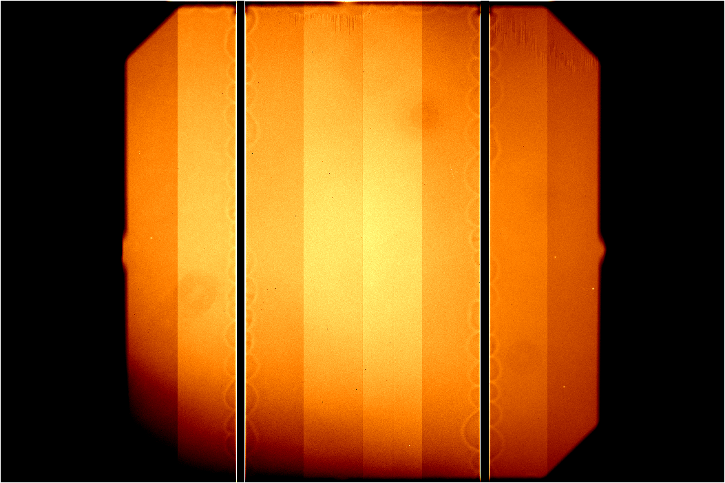
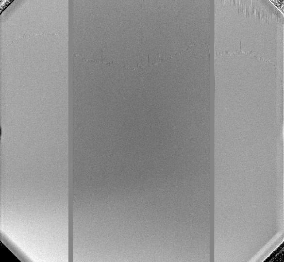
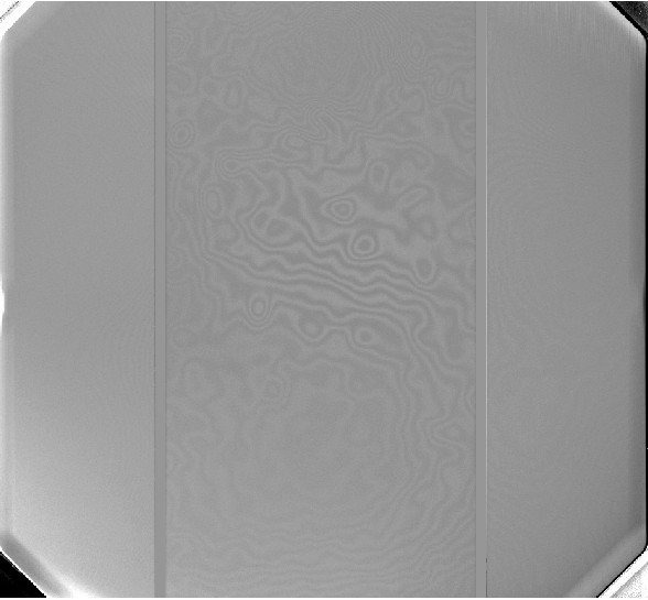
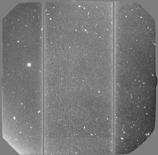
Single GMOS-N twilight flat frame taken through the r'-fitler in 2x2 binning and slow/low readout mode. The 12 amplifiers have been mosaiced without any bias subtraction. For this frame the partial obscuration caused by the air bubbles is most prominent in the lower left corner of the frame.
The air bubbles move with changes in telescope elevation and cass rotator angle, i.e. depending on the orientation of the GMOS collimator and camera lens groups with respect to the gravity vector. Since the oil is viscous, the bubbles have a long settling time of more than 30-40 min. For most configurations, the resulting obscuration will be prominent in the bottom part of the frame, but the exact location of the affected part is time-dependent. Typically, the bubble configuration and related obscuration will show small changes from frame to frame.
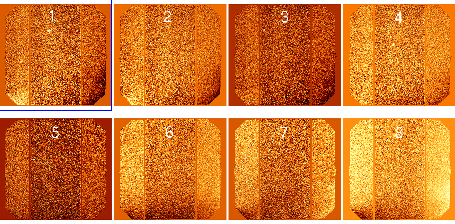
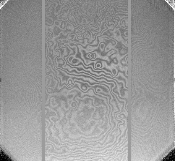
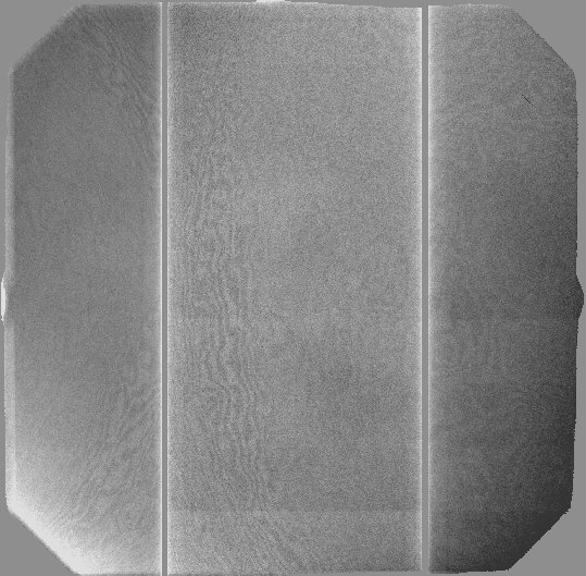
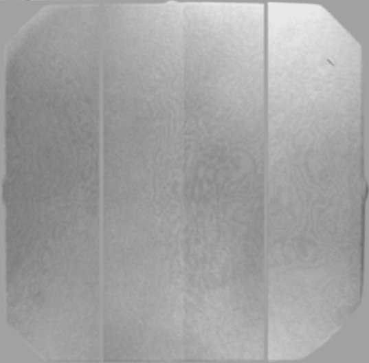
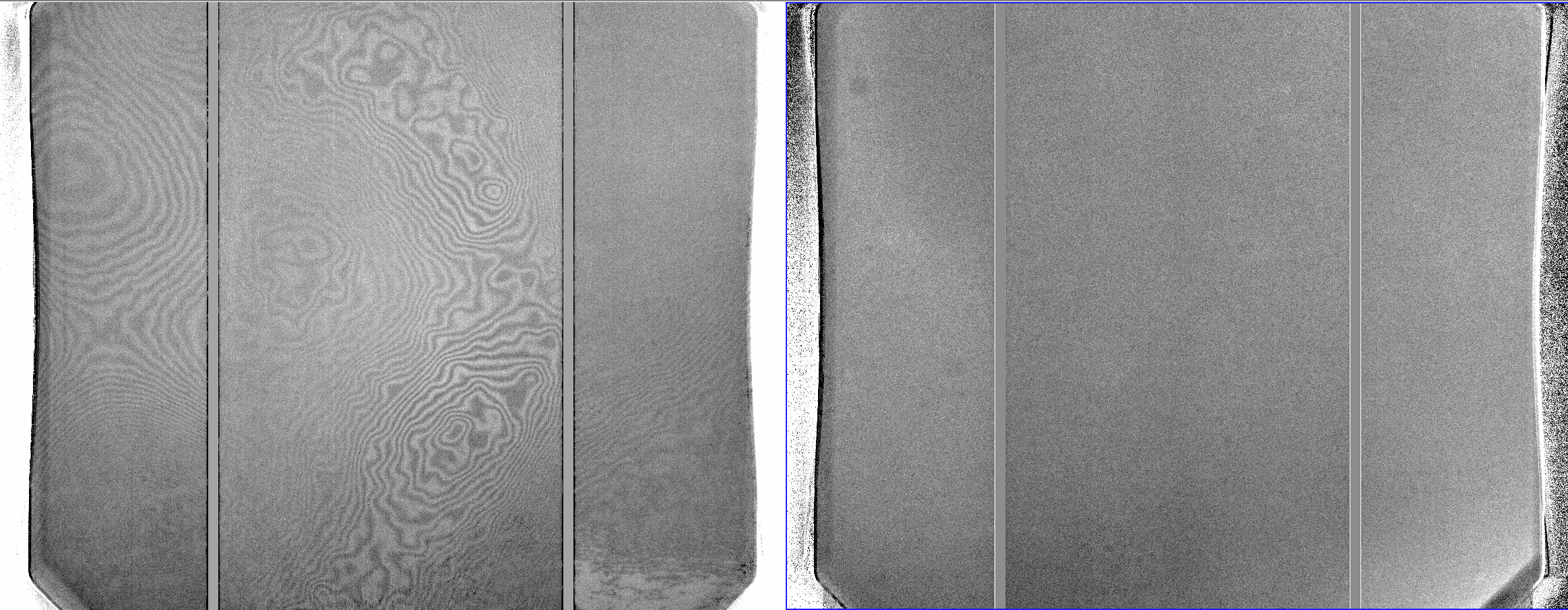
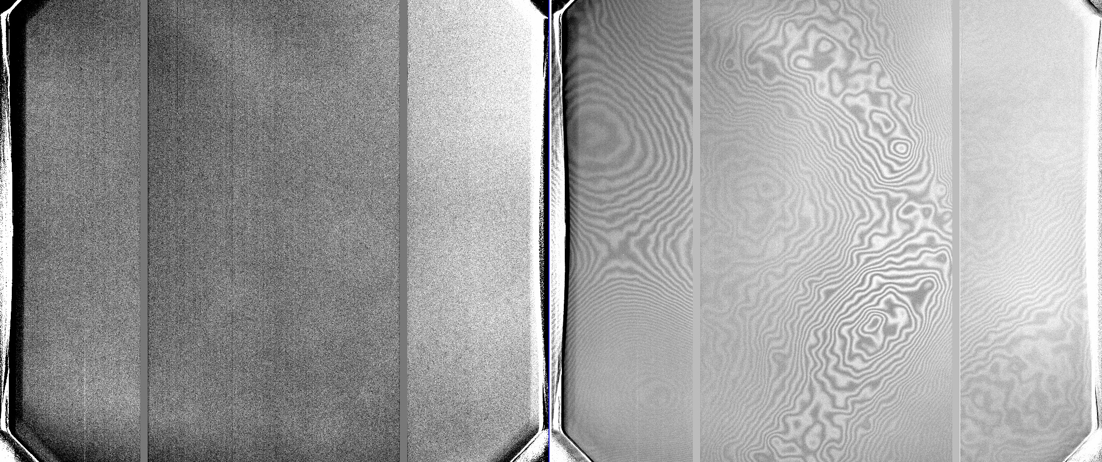
Eight consecutive i-band twilight flat exposures (labeled 1 to 8) after bias subtraction and flat fielding. The flat fielding is based on the average flat obtained by combining all eight exposures. Residuals after flat fielding due to the changing bubble configuration are most obvious in the lower left and right part of the frame. All eight consecutive twilight flat exposures were observed within less than 10 min. The images are not normalized and each color scale was chosen individually to highlight the residuals after flat fielding. (Note that these example twilight flats were taken in March 2018, during a period when GMOS-N was affected by a particularly extended air bubble after one of the collimator lens groups had suffered a major oil leak. While this lens group could be refilled with oil on 7 June 2018, less extended air bubbles in other lens groups remain.)
Effects on GMOS data
The main effect of the air bubbles is an obscuration of light usually towards the lower part of the frame. The obscuration pattern can differ from exposure to exposure, depending on the telescope elevation and cass rotator angle and the long oil settling time. As a result, morning twilight flats may show a very different obscuration pattern than imaging exposures obtained in a different part of the sky at night.
Tests with a GCAL-illuminated pinhole grid mask in GMOS-N have demonstrated that the parts of the frame affected by the air bubbles show a degraded pinhole image quality in addition to light obscuration. Whether the same applies to on-sky data and whether the air bubbles can affect astrometric accuracy is currently under investigation.
Data reduction/observing strategies
The obscuration caused by the changing bubble configurations in the GMOS lenses can limit the flat fielding accuracy, in particular in imaging mode. The following recommendations may help to improve flat fielding during data reduction.
- Dark sky flat fields: Imaging programs are recommended to use a sufficient number of dithers, so that the imaging exposures themselves can be combined into a dark sky flat. The dark sky flat will provide the best-possible match to the air bubble configuration in the science data. This strategy may not be viable for programs targeting very extended objects.
-
For very extended objects, the best option is to include some off-target sky exposures in the science sequences, analogously to the case of NIR imaging. This strategy has proven to be effective with GMOS-S. Taking at least three dithered sky frames of a nearby field with a low density of bright sources is what gives the best results.
-
Twilight flat exposures: Twilight flats are typically observed in morning twilight using a range of telescope elevations (header keyword ELEVATIO) and cass rotator angles (header keyword CRPA). In order to enhance the flat fielding accuracy, it is recommended to select the subset of twilight flat exposures that most closely matches the obscuration pattern in the imaging frames. (Note that frames with matching elevation and cass rotator angle do not necessarily provide the best match in terms of the bubble obscuration due to the long settling time of the index-matching oil. A visual selection of matching twilight flats may be required.)
PIs of GMOS-N/GMOS-S programs who encounter issues with the data calibration or have questions about the best observing strategies are welcome to contact the GMOS-N or GMOS-S science teams at gmos_n_science 'at' gemini.edu or gmos_s_science 'at' gemini.edu.
Flatfield Features
GMOS-N flatfield features introduced with the Hamamatsu CCDs
There are a number of new flatfield features seen in the GMOS-N Hamamatsu CCDs commissioned in 2017A. There is currently less dust visible in the field than with the previous arrays, and there is no longer a "dust bunny" feature (see below).
GMOS-N flatfield features introduced during August 2006 shutdown
August 30, 2006
GMOS-N was removed from the telescope July 31, 2006 as part of an extensive Gemini North shutdown period. GMOS-N was mounted on the telescope (port 5, same as previously) again on August 9. The first science data was obtained the evening of August 16 (UT August 17).
Unfortunately, at some point during this time a large flatfield feature was introduced into the GMOS-N optical path. A series of tests has determined that this feature:
- extinguishes ~2.5-3% of the incident light at the darkest point
- is present in all filters
- does not move around with either telescope position or cass rotator angle
- is located within GMOS-N somewhere downstream of the grating/mirror turret
- is not located on the detector package
- is most likely located within the GMOS-N camera
- appears to flatfield out quite well when appropriate twilight flats are used
- does not flatfield out when domeflats are used
It is very important that GMOS-N users take care to use appropriate baseline twilight flats when reducing their data: All GMOS-N data taken since and including August 17, 2006 UT should be flatfielded with twilight flats also obtained after and including August 17, 2006 UT.
Further details and images are provided below. Please note that, while we suspect that this feature arises from dust somewhere in the camera, the affectionate term "dustbunny" is not intended to imply that we actually are aware of the nature of the substance causing the new GMOS-N flatfield feature as yet.
- GMOS-N r-band and i-band 2x2 Twilight Flats showing the dustbunny
- GMOS-N r-band imaging data of an unidentified field flatfielded with improper and proper Twilight Flats
- GMOS-N i-band imaging data of an unidentified field flatfielded with improper and proper Twilight Flats
Fringing
The GMOS-N and GMOS-S EEV detectors had significant fringing in the red. The GMOS-N DD E2V detectors, which were in operation until February 2017, and the new GMOS-N and GMOS-S Hamamatsu detectors exhibit much less fringing than the original EEV detectors. The pages in this section show examples of fringe frames in imaging mode as well as science data before and after correction for fringing.
Gemini North
The GMOS-N E2V DD CCDs, used between Nov 2011 and Feb 2017, had much weaker fringing than the original GMOS-N EEV CCDs or the new Hamamatsu CCDs. This page shows examples of fringe frames in imaging mode.
Raw fringe frames for i', Z, z', and Y filters can be downloaded from the Gemini Observatory Archive. To retrieve fringe frames taken with the EEV and DD E2V CCDs since 2009, please search for Target Name "Fringe Frame". (Please note that the DD E2V CCDs were installed in Nov 2011 and replaced by the Hamamatsu detectors in February 2017.)
To retrieve fringe frames taken with the Hamamatsu detectors, please specify Target Name "Blankfield".
(Note that filenames beginning with RG and _FRINGE in the Data Label indicate processed frames.)
Hamamatsu CCDs:
The Hamamatsu CCDs for GMOS-N have similar fringing properties as observed for the GMOS-S Hamamatsu CCDs. Fringing is negligible in i' and Z filters. Fringing is noticeable in z' and Y filters. The worst fringing is in the middle chip, at the level of about 1% of the background in z' and almost 2% on average in Y. Below we show fringe frames for i' (top left), Z (top right), z' (bottom left), and Y (bottom right) at the same scaling. These were taken in March-April 2017. We highly recommend for z' and Y imaging to take enough dithers to generate your own fringe frames.
 |
 |
 |
 |
![Chart showing Relative Fringe Strength vs Column [pix] for z' and Y filters](http://www.gemini.edu/sciops/instruments/gmos/FringeYzHam.jpg)
Upgraded E2V DD CCDs:
The data shown for the E2V DD CCDs were taken between Dec 2011 - Feb 2012, on photometric nights in dark time. Fringing in the z'-filter is typically +-0.3% of the background, while the i'-filter fringing is less than +- 0.15% of the background.
 |
 |
|
z'-filter fringe frame. |
i'-filter fringe frame, median filtered with a box 17 pixels by 17 pixels in order to increase the signal-to-noise to make the fringes more apparent. |
A z'-band science frame without fringe subtraction. Note the fringing is much weaker than in the original EEV CCDs as shown above.
A comparison of z'-band fringing between the original and upgraded EEV CCDs:
This shows a cut along a single column. Fringing in the DD E2V CCDs in the z'-band is about a tenth as strong as in the original EEV CCDs.
The original EEV CCDs
The data shown for the original EEV CCDs were obtained the night of August 19-20, 2001, during the commissioning of GMOS-N. This was close to new moon, and the sky was photometric. The fringe strength in the z'-filter is typically +-2.5% of the background, while in the i'-filter the fringing is +-0.7% of the background.
 |
 |
|
z'-filter fringe frame. |
i'-filter fringe frame. The images was median filtered with a box 17pixels by 17 pixels in order to increase the signal-to-noise. Because this fringe frame was constructed from only 6 science exposures, artifacts are seen from insufficient cleaning of signal from objects. The signal in the artifacts is typically less than 1% of the background level. |
Relative strength of the fringes in the z'- and the i'-filter.
 |
 |
z'-filter science frame before and after fringe subtraction.
 |
 |
i'-filter science frame before and after fringe subtraction.
Gemini South
The new GMOS-S Hamamatsu CCDs have significantly less fringing than the EEV detectors. The fringing in i' is negligible (compared to the ~67% in i' on the EEVs), as well as in CaT and Z; about 1% in z' and ~2.5% in Y. Example snapshots below show z' band (top left), i'(top right), Z (bottom left) and Y (bottom right) fringe frames.
------------
The GMOS-S EEV (no longer available) CCDs have significant fringing in the red. This page shows examples of fringe frames in imaging mode in the i'-filter and the z'-filter as well as science data before and after correction for the fringing.
Recent fringe frames for both i' and z' are available from the Gemini Science Archive. To retrieve either the raw or the processed frames one can follow these steps (eg.):
- - Under GSA Queries select menu item Search Complete Catalogue
- - Select a Standard Query GMOS-N and/or GMOS-S and click Continue to query form...
- - In Target Name enter Fringe and from the Resolver: menu select Gemini name (not the default value SIMBAD/NED). Alternatively, in Data Label choose "Contains" and enter fringe
- - in Filters enter either i_G0327 or z_G0328
- - From the Instrument menu select GMOS-S
- - In CCDSUM enter either 1 1 or 2 2
- - Select the raw or processed frames you wish to retrieve and continue by clicking Download Datasets. Note the processed frames have _fringe in the Data Label and the filename begins with RG.
Imaging Fringe Frames are taken on a one-set-per-semester basis. The ones shown below were obtained in November/December 2010 and the corresponding processed fringe frames area available through the GSA. The latest fringe frames were observed on 2013A and are being processed.
 |
 |
|
z'-filter fringe frame. |
i'-filter fringe frame. |
Example of science data before and after correction for the fringing. The data were obtained the night of May 24-25, 2003 during the commissioning of GMOS-S. The images are from dataset GS-2003A-SV-228.
 |
 |
i'-filter science frame before and after fringe subtraction.
Last update: November 19, 2014; German Gimeno
Scattered Light
Both GMOS-N and GMOS-S suffer fairly significant scattered light in spectroscopic mode. The six gratings exhibit different levels of scattered light, with some gratings being more affected by red scattered light than blue (some examples shown below). The scattered light affects both science observations and GCAL lamp (flat and CuAr) calibration exposures. Note that the GCALflat lamp is very red, and scattered light from astronomical sources will have different relative strengths of blue and red scattered light depending on their intrinsic spectral properties.
The two dimensional shape of the scattered light is rather smooth and spatially fills the entire detector, as can be seen from the example images below. The result of this is that a faint science target can suffer significant contamination from a much brighter object within the GMOS field of view (eg. bright objects also falling on the longslit or bright alignment targets in MOS masks). Because the scattered light character is spatially smooth it is removed fairly adequately as part of the sky subtraction procedure, but the increased Poisson noise can negatively impact the final signal-to-noise of the science target. This is particularly a concern for very faint targets observed in the blue during new moon, when the nominal sky background is very low.
In order to minimize the effects of scattered light from other bright targets one may wish to consider one of the following strategies:
- Avoid placing much brighter objects on the slit, IFU, or MOS slitlet with your science target if there is no scientific reason to include them.
- For MOS, it may be beneficial to include an offset iterator in your science observation to offset the field a small amount (eg. q=5 arcsec) after the mask is aligned in order to move the alignment stars out of their 2 arcsec wide boxes. If adopting this strategy it is essential to ensure that either the MOS science slitlets have sufficient length to accommodate the offset or employ the corresponding y-offset to the science targets when designing the MOS mask.
- If you need to check how scattered light looks for a particular configuration, you may fetch the specific configuration desired from the archive or request an advance test flat be obtained for your program.
Unfortunately, there is little that can be done to avoid scattered light from the science target itself, particularly when observing with the lower resolution gratings. For the higher resolution gratings, it may be advantageous to observe through a broadband filter in order to avoid scattered light contamination from wavelengths beyond the region of scientific interest. Any of these strategies should be adopted with care, we recommend you consult with your contact scientist or the GMOS-N/S instrument scientist if you are concerned with minimizing the effects of spectroscopic scattered light on your science data.
The following images illustrate the spatial distribution of scattered light in longslit spectral images from a single bright star. Both a red star and a blue star were observed on two separate occasions, these data all used the B600 grating.
| EG131 (blue star) | ||||
| Central Wavelength 400nm (262 - 538 nm) | ||||
| no filter | g-filter | r-filter | i-filter | z-filter |
![[EG131 B600 400nm no filter]](http://www.gemini.edu/sciops/instruments/gmos/B600n_400nm_none_bluestar.jpg "EG131 B600 400nm no filter.") |
![[EG131 B600 400nm r filter]](http://www.gemini.edu/sciops/instruments/gmos/B600n_400nm_r_bluestar.jpg "EG131 B600 400nm r filter.") |
![[EG131 B600 400nm i filter]](http://www.gemini.edu/sciops/instruments/gmos/B600n_400nm_i_bluestar.jpg "EG131 B600 400nm i filter.") |
![[EG131 B600 400nm z filter]](http://www.gemini.edu/sciops/instruments/gmos/B600n_400nm_z_bluestar.jpg "EG131 B600 400nm z filter.") |
|
| Central Wavelength 900nm (762 - 1038 nm) | ||||
![[EG131 B600 900nm no filter]](http://www.gemini.edu/sciops/instruments/gmos/B600n_900nm_none_bluestar.jpg "EG131 B600 900nm no filter.") |
![[EG131 B600 900nm g filter]](http://www.gemini.edu/sciops/instruments/gmos/B600n_900nm_g_bluestar.jpg "EG131 B600 900nm g filter.") |
![[EG131 B600 900nm r filter]](http://www.gemini.edu/sciops/instruments/gmos/B600n_900nm_r_bluestar.jpg "EG131 B600 900nm r filter.") |
||
| HD195275 (red star) | ||||
| Central Wavelength 400nm (262 - 538 nm) | ||||
| no filter | g-filter | r-filter | i-filter | z-filter |
![[HD195275 B600 400nm no filter]](http://www.gemini.edu/sciops/instruments/gmos/B600o_400nm_none_redstar.jpg "HD195275 B600 400nm no filter.") |
![[HD195275 B600 400nm r filter]](http://www.gemini.edu/sciops/instruments/gmos/B600o_400nm_r_redstar.jpg "HD195275 B600 400nm r filter.") |
![[HD195275 B600 400nm i filter]](http://www.gemini.edu/sciops/instruments/gmos/B600o_400nm_i_redstar.jpg "HD195275 B600 400nm i filter.") |
![[HD195275 B600 400nm z filter]](http://www.gemini.edu/sciops/instruments/gmos/B600o_400nm_z_redstar.jpg "HD195275 B600 400nm z filter.") |
|
| Central Wavelength 900nm (762 - 1038 nm) | ||||
![[HD195275 B600 900nm no filter]](http://www.gemini.edu/sciops/instruments/gmos/B600o_900nm_none_redstar.jpg "HD195275 B600 900nm no filter.") |
![[HD195275 B600 900nm g filter]](http://www.gemini.edu/sciops/instruments/gmos/B600o_900nm_g_redstar.jpg "HD195275 B600 900nm g filter.") |
![[HD195275 B600 900nm r filter]](http://www.gemini.edu/sciops/instruments/gmos/B600o_900nm_r_redstar.jpg "HD195275 B600 900nm r filter.") |
||
Scattered light longslit B600 spectral images arising from a single bright star. Click to view full images.
The following two sets of images illustrate the relative contribution of scattered light from GCALflat data. All data were taken using identical GCAL configurations and exposure times. The B600, R400 and gratings are compared at both red and blue central wavelengths. Because the GCAL flat lamp is very red the effect of red scattered light in blue data is much more noticeable than the effect of blue scattered light in red data for both gratings. Because identical configurations and display stretches are used one can see how the B600 grating is more affected by red scattered light than the R831 grating.
| B600 grating | ||||
| Central Wavelength 400nm (262 - 538 nm) | ||||
| no filter | g-filter | r-filter | i-filter | z-filter |
![[GCALflat B600 400nm no filter]](http://www.gemini.edu/sciops/instruments/gmos/B600_400_none_GCALflat.jpg "GCALflat B600 400nm no filter.") |
![[GCALflat B600 400nm g filter]](http://www.gemini.edu/sciops/instruments/gmos/B600_400_g_GCALflat.jpg "GCALflat B600 400nm g filter.") |
![[GCALflat B600 400nm r filter]](http://www.gemini.edu/sciops/instruments/gmos/B600_400_r_GCALflat.jpg "GCALflat B600 400nm r filter.") |
![[GCALflat B600 400nm i filter]](http://www.gemini.edu/sciops/instruments/gmos/B600_400_i_GCALflat.jpg "GCALflat B600 400nm i filter.") |
![[GCALflat B600 400nm z filter]](http://www.gemini.edu/sciops/instruments/gmos/B600_400_z_GCALflat.jpg "GCALflat B600 400nm z filter.") |
| Central Wavelength 850nm (712 - 988 nm) | ||||
![[GCALflat B600 850nm no filter]](http://www.gemini.edu/sciops/instruments/gmos/B600_850_none_GCALflat.jpg "GCALflat B600 850nm no filter.") |
![[GCALflat B600 850nm g filter]](http://www.gemini.edu/sciops/instruments/gmos/B600_850_g_GCALflat.jpg "GCALflat B600 850nm g filter.") |
![[GCALflat B600 850nm r filter]](http://www.gemini.edu/sciops/instruments/gmos/B600_850_r_GCALflat.jpg "GCALflat B600 850nm r filter.") |
![[GCALflat B600 850nm i filter]](http://www.gemini.edu/sciops/instruments/gmos/B600_850_i_GCALflat.jpg "GCALflat B600 850nm i filter.") |
![[GCALflat B600 850nm z filter]](http://www.gemini.edu/sciops/instruments/gmos/B600_850_z_GCALflat.jpg "GCALflat B600 850nm z filter.") |
| R400 grating | ||||
| Central Wavelength 400nm (192 - 608 nm) | ||||
| no filter | g-filter | r-filter | i-filter | z-filter |
![[GCALflat R400 400nm no filter]](http://www.gemini.edu/sciops/instruments/gmos/R400_400_none_GCALflat.jpg "GCALflat R400 400nm no filter.") |
![[GCALflat R400 400nm g filter]](http://www.gemini.edu/sciops/instruments/gmos/R400_400_g_GCALflat.jpg "GCALflat R400 400nm g filter.") |
![[GCALflat R400 400nm r filter]](http://www.gemini.edu/sciops/instruments/gmos/R400_400_r_GCALflat.jpg "GCALflat R400 400nm r filter.") |
![[GCALflat R400 400nm i filter]](http://www.gemini.edu/sciops/instruments/gmos/R400_400_i_GCALflat.jpg "GCALflat R400 400nm i filter.") |
![[GCALflat R400 400nm z filter]](http://www.gemini.edu/sciops/instruments/gmos/R400_400_z_GCALflat.jpg "GCALflat R400 400nm z filter.") |
| Central Wavelength 850nm (642 - 1058 nm) | ||||
![[GCALflat R400 850nm no filter]](http://www.gemini.edu/sciops/instruments/gmos/R400_850_none_GCALflat.jpg "GCALflat R400 850nm no filter.") |
![[GCALflat R400 850nm g filter]](http://www.gemini.edu/sciops/instruments/gmos/R400_850_g_GCALflat.jpg "GCALflat R400 850nm g filter.") |
![[GCALflat R400 850nm r filter]](http://www.gemini.edu/sciops/instruments/gmos/R400_850_r_GCALflat.jpg "GCALflat R400 850nm r filter.") |
![[GCALflat R400 850nm i filter]](http://www.gemini.edu/sciops/instruments/gmos/R400_850_i_GCALflat.jpg "GCALflat R400 850nm i filter.") |
![[GCALflat R400 850nm z filter]](http://www.gemini.edu/sciops/instruments/gmos/R400_850_z_GCALflat.jpg "GCALflat R400 850nm z filter.") |
| R831 grating | ||||
| Central Wavelength 400nm (296 - 504 nm) | ||||
| no filter | g-filter | r-filter | i-filter | z-filter |
![[GCALflat R831 400nm no filter]](http://www.gemini.edu/sciops/instruments/gmos/R831_400_none_GCALflat.jpg "GCALflat R831 400nm no filter.") |
![[GCALflat R831 400nm g filter]](http://www.gemini.edu/sciops/instruments/gmos/R831_400_g_GCALflat.jpg "GCALflat R831 400nm g filter.") |
![[GCALflat R831 400nm r filter]](http://www.gemini.edu/sciops/instruments/gmos/R831_400_r_GCALflat.jpg "GCALflat R831 400nm r filter.") |
![[GCALflat R831 400nm i filter]](http://www.gemini.edu/sciops/instruments/gmos/R831_400_i_GCALflat.jpg "GCALflat R831 400nm i filter.") |
![[GCALflat R831 400nm z filter]](http://www.gemini.edu/sciops/instruments/gmos/R831_400_z_GCALflat.jpg "GCALflat R831 400nm z filter.") |
| Central Wavelength 850nm (746 - 954 nm) | ||||
![[GCALflat R831 850nm no filter]](http://www.gemini.edu/sciops/instruments/gmos/R831_850_none_GCALflat.jpg "GCALflat R831 850nm no filter.") |
![[GCALflat R831 850nm g filter]](http://www.gemini.edu/sciops/instruments/gmos/R831_850_g_GCALflat.jpg "GCALflat R831 850nm g filter.") |
![[GCALflat R831 850nm r filter]](http://www.gemini.edu/sciops/instruments/gmos/R831_850_r_GCALflat.jpg "GCALflat R831 850nm r filter.") |
![[GCALflat R831 850nm i filter]](http://www.gemini.edu/sciops/instruments/gmos/R831_850_i_GCALflat.jpg "GCALflat R831 850nm i filter.") |
![[GCALflat R831 850nm z filter]](http://www.gemini.edu/sciops/instruments/gmos/R831_850_z_GCALflat.jpg "GCALflat R831 850nm z filter.") |
Scattered light MOS B600 and R831 spectral images corresponding to GCALflats centered on 400 and 850nm. The MOS mask consists of two widely separated (in y) slitlets (centered in x). The scattered light images in blue light are very faint, mainly due to the lack of blue light in the GCAL flat lamp. The scattered red light images are very smooth for blue central wavelengths, though for red central wavelengths they show some structure both spatially and in wavelength implying that some fraction of the scattered light contribution is dispersed light. All exposures were 120s long using the ND4-5 filter in GCAL. All images are displayed with the same stretch to reveal the difference in scattering between the two gratings. Click to view full images.