Each new calculation will post results into the same page. The results page can be printed and re-sized e.g. so that the ITC form and results are both visible on your screen.
Additional information is available for:
- Image size and aperture
- Format of imaging and spectroscopic results; saving spectra as ASCII files
- S/N calculations
- Error messages
Image Size and Aperture
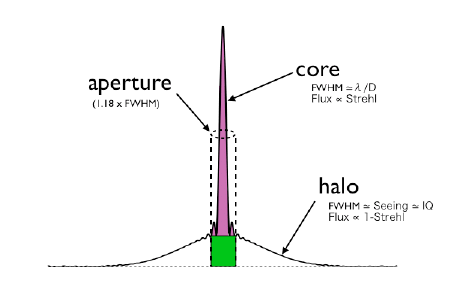
The derived image size (FWHM of the assumed Gaussian PSF) includes contributions from seeing, telescope diffraction, the performance of the tip-tilt secondary and many other components. See the image quality predictions in the observing condition constraints for more details of the wavelength dependence and frequency of occurrence. For the adaptive optics case both the FWHM of the AO-corrected core and the FWHM of the uncorrected halo are given, as is the Strehl ratio.
The "optimum aperture" size is described on the analysis methods page.
For most uniform surface brightness (USB) calculations, the (assumed circular) software aperture corresponds to an area of 1 arcsec^2 when the "optimum aperture" analysis option is selected. (A different value can be specified by the user and the point source size is also reported for reference). However in the case of the GMOS IFU, the "optimum aperture" option corresponds to a single IFU spatial element (not 1 arcsec^2) and the spectra from that IFU fiber (nominally 5 detector rows) are summed. No optimal extraction or deconvolution is performed at this time.
Format of imaging and spectroscopic results
In imaging calculations, the results page displays relevant derived properties on the top half page and key user parameters at the bottom. For spectroscopic calculations the relevant signal, noise and S/N characteristics are shown graphically.
If the final and single exposure S/N are the same then only the former is visible.
In the cross-dispersed mode with GNIRS, the source signal and sqrt(background) are color-coded for each order with dark and light shades of the same color. Only the final S/N plot (i.e. not the single-exposure chart) is shown.
To view (or save) the spectra as ASCII files with tab-separated columns, click (or shift+click) on the link(s) under each plot. The wavelength units are nm; the ordinate has the same units as the graphics plot.
Signal to noise calculations
See the calculation and analysis methods for more details on how the S/N for the whole observation is derived.
Error messages - most are self explanatory; others:
- Can't find sourceGeom - usually occurs when trying to use the ITC from Netscape 6.x which doesn't work with forms.
- Please use a model line width > 1 nm to avoid undersampling of the line profile when convolved with the transmission response - the ITC currently samples the sky transmission spectrum, background and many other optical elements at 0.25-0.5nm resolution. Hence any model emission line that is narrower than 1nm may not be correctly propagated through the calculator.
Calculation methods
There are two modes available:
- Calculate the total signal-to-noise ratio (S/N) for an observation with the specified exposure time, number of exposures and sky subtraction method
- Calculate the total integration time to achieve the requested S/N for an observation with the specified exposure time and sky subtraction method
As the S/N can vary markedly with wavelength, particular in the infrared, only the former mode is available for spectroscopic calculations.
The Integration Time Calculator reports the total signal and noise for a single exposure and the signal-to-noise ratio (S/N) for a single exposure and for the whole observation. In general, the theoretical S/N (reported by the ITC as the "intermediate S/N") for a single exposure is not achievable because it is necessary to perform sky or background subtraction. In practice there are many ways to achieve this subtraction depending on the frequency of sky observations, the spatial extent of the object (e.g. it may be necessary to observe separate sky frames in a crowded field or for an extended object) and the personal preference of the observer.
The ITC uses an approximation that each on-source exposure measures both signal and noise and that the process of background subtraction adds another contribution of noise. (This is a generally applicable case; it can be shown that this approximation is within 0.5 to sqrt(3) of other approaches to background subtraction). In this case the final S/N is:
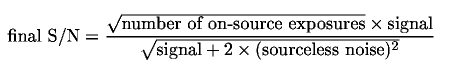
where "aperture ratio" is (1 + source aperture area / sky aperture area). For some instruments the aperture ratio may be defined by the user in the ITC; in others (e.g. NIRI) it is fixed equal to unity at present. The 'sourceless noise' is defined as the (quadratic) combination of background, readout and dark current noise:
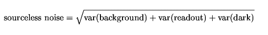
where var(background) is the square of the background noise (i.e. the background flux) etc. and the number of on-source exposures is:
![]()
Several examples should clarify the behaviour of this algorithm. In each case we assume that the source is faint so that the observation is (sky + telescope) background noise limited and set the aperture ratio to 2.
- Let the total number of exposures be 1. The ITC reports a final S/N that is worse than that derived intrinsically for the single exposure because it assumes background subtraction mst be performed.
- Let the total number of exposures be 4 all of which are on-source (e.g. we have offset the telescope but kept the target within the detector or slit field of view). The on-source integration time is 4t. The final S/N is sqrt(2) better than an observation with 2 exposures (integration time 2t) as we have doubled the on-source integration time.
- Let the total number of exposures be 4 but only 2 of which are on-source (e.g. we have offset the telescope to blank sky because the source is large or are chopping and nodding off-chip). The on-source integration time is 2t. The final S/N is sqrt(2) worse than case (2) and the same as an observation with 2 on-source exposures.
Analysis methods
For imaging and slit spectroscopy modes there are two methods available to estimate the signal and noise for the input source given the observational setup:
- Emply a software aperture optimised to yield the best S/N ratio (i.e., "optimum extraction")
- Employ an aperture specified by the user
The optimum aperture differs slightly for bright and faint sources (i.e. it depends on the dominant source of noise) but an effective compromise over a wide range of source brightness is 1.18 * FWHM for imaging a point source (see the notes associated with the IRAF routine noao.astutil.ccdtime for further information). This aperture contains 61% of the total signal for the assumed Gaussian PSF. (See the more details of the default aperture used in the AO case).
In the case of a uniform surface brightness (USB) source the optimum aperture simply defaults to an area of one square arcsec. Depending on the dominant source of noise, larger apertures will typically give higher S/N in the USB case.
For spectroscopy, the equivalent length integrated along the major axis (i.e., spatial axis) of the slit that yields the best S/N ratio would be 1.4 * FWHM for a Gaussian PSF. For computational simplicity, the ITC rounds this length to an integer number of pixels.
When calculating the area enclosed by the software aperture in the imaging case, the minimum is 9 pixels.
The ITC results page reports the aperture used by the software, the fraction of the source flux it contains and the source + background signal in the peak pixel.
For IFU modes there are three analysis methods available to estimate the signal and noise of your source:
- Calculate the signal and noise for a single element (i.e., spaxel) offset by a specified number of arcseconds from the source center
- Calculate the signal and noise for an aperture consisting of the specified number of elements and centered on the source
- Calculate the signal and noise per element over a specified range from the source center (negative values are valid, though all sptial profiles are azimuthally symmetric)
The first two methods will provide a single set of plots: signal and background per individual spaxel for a single integration as well as the S/N in a single exposure and all exposures combined across all elements (if more than one is specified). The third method will provide a series of plots, one pair for each element specified. Input numbers are rounded to the nearst integer number of elements.
Last update May 4, 2023; Brian C. Lemaux and Andrew Stephens
Definition of an Astronomical Source in the ITC
Definition of an astronomical source involves specification of the spatial profile, the brightness normalisation and the spectrum.
Spatial profile
The astronomical target may be a point or an extended source.
The nominal point source has a size defined by the image quality constraint and air mass (selected as part of the observing conditions), the wavelength (selected by the colour filter or dispersive element as part of the instrument properties) and the wavefront sensor (selected as part of the telescope properties). The adopted extent of the point source (in arcsec) is reported in the ITC results.
Several different extended sources are available. Currently a 2-dimensional Gaussian profile with user-defined FWHM (in arcsec) and an extended source with uniform surface brightness may be selected. The user-defined FWHM is defined as the image size delivered in the telescope focal plane (i.e. it includes seeing). An arbitrary spatial profile imported from an external file will be available at a later date.
Source brightness and units
The source flux density or, for uniform extended sources, surface brightness are specified in familiar astronomical units available via the pull-down menus. The source brightness is converted into the ITC internal units of photons/s/nm/m^2 (optionally, per square arcsec) using the relationships described below. The source brightness can be specified at a wavelength that is not the observing wavelength provided that the chosen (redshifted) spectrum extends across the entire wavelength range of interest (e.g. that defined by the colour filter).
(a) mag
Zero points giving continuum photons/s/nm/m^2 for a zero magnitude source are assumed to be:
| Waveband | Wavelength (um) | Zeropoint (photons/s/nm/m^2) |
| U | 0.36 | 7.59 * 10^7 |
| B | 0.44 | 1.46 * 10^8 |
| g' | 0.48 | 1.27 * 10^8 |
| V | 0.55 | 9.71 * 10^7 |
| r' | 0.62 | 1.08 * 10^8 |
| R | 0.67 | 6.46 * 10^7 |
| i' | 0.77 | 9.36 * 10^7 |
| I | 0.87 | 3.90 * 10^7 |
| z' | 0.92 | 7.98 * 10^7 |
| J | 1.25 | 1.97 * 10^7 |
| H | 1.65 | 9.6 * 10^6 |
| K | 2.20 | 4.5 * 10^6 |
| L' | 3.76 | 9.9 * 10^5 |
| M' | 4.77 | 5.1 * 10^5 |
| N | 10.5 | 5.1 * 10^4 |
| Q | 20.1 | 7.7 * 10^3 |
These values were derived from the CIT system used in the STScI units conversion tool (UBVRI), Cohen et al. (1992. AJ, 104, 1650; JHKL'M' from Vega and Sirius for 10 and 20um), and Schneider, Gunn, & Hoessel (1983; g', r', i', z').
(b) AB mag
The photon flux density (in photons/s/nm/m^2) as a function of the source brightness in AB magnitudes is given by:
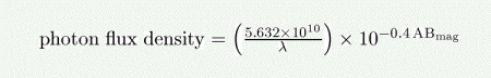
where lambda is the wavelength in nm. This is equivalent to the formal definition in Oke & Gunn (1983. ApJ, 266, 713).
(c) Jy
The photon flux density (in photons/s/nm/m^2) as a function of the source brightness in Jy (i.e. 10^-26 W/m^2/Hz) is given by:
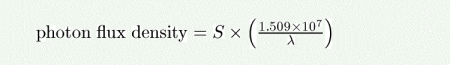
where lambda is the wavelength in nm.
(d) W/m^2/um
The photon flux density (in photons/s/nm/m^2) as a function of the source brightness in W/m^2/um is given by:
where lambda is the wavelength in nm.
(e) ergs/s/cm^2/Angstrom
The photon flux density (in photons/s/nm/m^2) as a function of the source brightness in ergs/s/cm^2/Angstrom is given by:
where lambda is the wavelength in nm.
(f) ergs/s/cm^2/Hz
The photon flux density (in photons/s/nm/m^2) as a function of the source brightness in ergs/s/cm^2/Hz is given by:
where lambda is the wavelength in nm.
Spectral distribution
The source spectrum is selected from the available libraries of stellar and non-stellar spectra, model emission line + continuum, and black body, power law and user-defined spectra. Different options are available depending on the instrument in question. The spectrum may be redshifted by an arbitrary amount. If the selected (redshifted) spectrum does not completely cover the observing wavelength range, as defined by the colour filter or dispersive element, either an error is reported by the ITC or the spectrum is padded with leading or trailing zeros.
For spectroscopic calculations, the source spectrum is smoothed to the resolution of the spectrograph as given by the dispersing element with an entrance aperture defined by the slit width, or source extent if narrower (some exceptions are noted for specific instruments). Note that the stellar and non-stellar libraries may have an intrinsic resolution less than that of the instrument or a coarser sampling. In all cases they are re-sampled to the appropriate dispersion within the ITC.
The sky transmission and sky background spectra employed currently have a resolution of ~1nm and sampling of ~0.5nm. Hence at higher instrument spectral resolutions, the sky lines will not be treated correctly.
(a) Non-stellar library
Rest-frame optical and near-IR spectra:
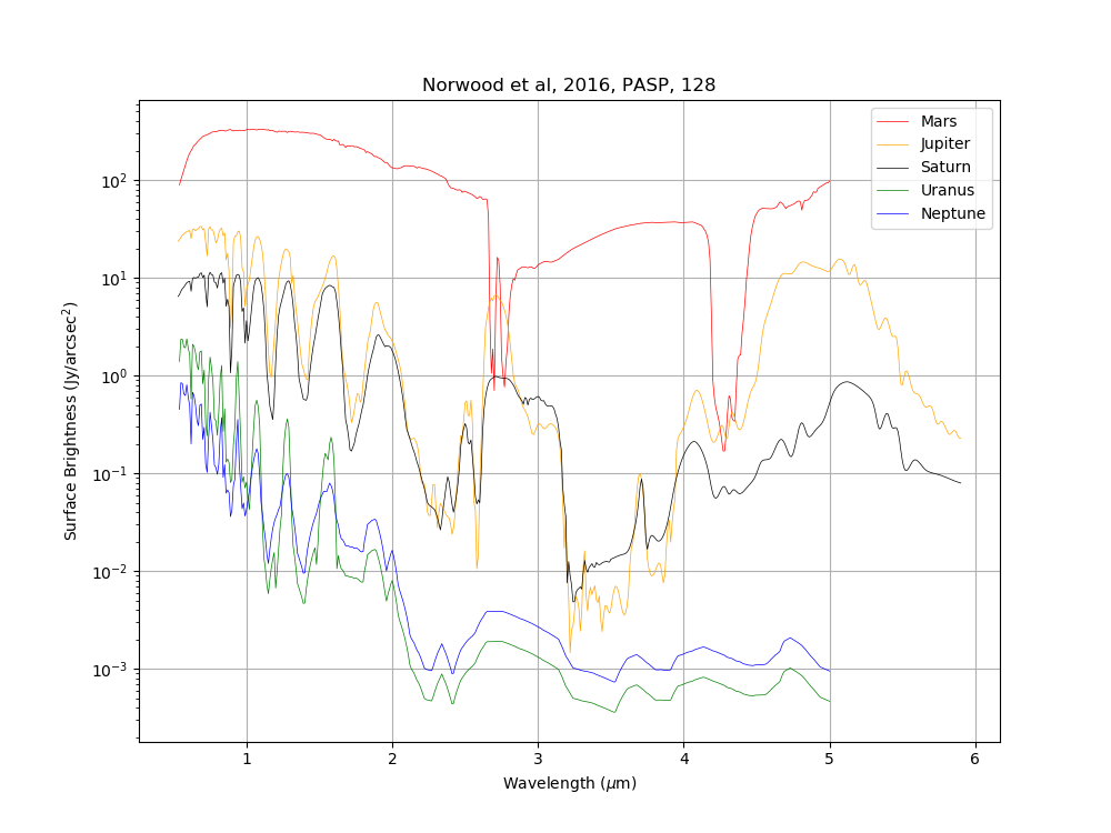
- Mars [plot, pata] is a composite spectrum from Norwood et al, 2016, PASP, 128, 25004 using the visible to near-IR albedo spectrum from McCord, T. B., Elias, J. H., & Westphal, J. A. 1971, Icar, 14, 245, and the 2.5 - 5 micron ISO spectrum from Lellouch, E., Encrenaz, T., de Graauw, T., et al. 2000, P&SS, 48, 1393.
- Jupiter and Saturn [plot, Jupiter data, Saturn data] are composite spectra from Norwood et al, 2016, PASP, 128, 25004 using the visible to near-IR albedo spectra from Clark, R. N., & McCord, T. B. 1979, Icar, 40, 180, the visible to 1 micron geometric albedo spectrum from Karkoschka, E. 1994, Icar, 111, 174, and the 2.5 - 5 micron ISO spectrum from Encrenaz, T., Lellouch, E., Feuchtgruber, H., et al. 1997, in Proc. First ISO Workshop on Analytical Spectroscopy, ESA-SP, 419, 125.
- Uranus and Neptune [plot, Uranus data, Neptune data] are composite spectra from Norwood et al, 2016, PASP, 128, 25004 using the visible to near-IR albedo spectra from Fink, U., & Larson, H. P. 1979, ApJ, 233, 1021, the visible to 1 micron geometric albedo spectra from Karkoschka, E. 1994, Icar, 111, 174, the 2.5 - 5 micron Akari albedo spectrum of Neptune (scaled for Uranus) from Burgdorf, M. J., Drossart, P., Encrenaz, T., Fletcher, L. N., & Orton, G. 2008, BAAS, 40, 489, and the 2.6-4um ISO spectra from Encrenaz, T., Lellouch, E., Feuchtgruber, H., et al. 1997, in Proc. First ISO Workshop on Analytical Spectroscopy, ESA-SP, 419, 125.
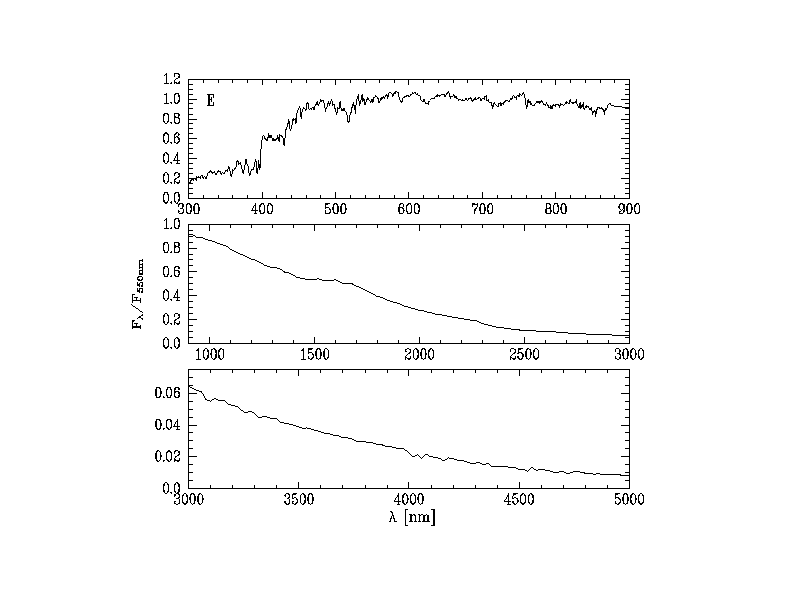
- Elliptical galaxy [plot, data] is a template spectrum (class T=-5, -4) covering the wavelength range 22 - 10000 nm and taken from the Pegase Atlas of Galaxies by Fioc & Rocca-Volmerange, 1997, A&A, 326, 950F. The spectrum has a sampling of 1nm at wavelengths shortwards of 878nm and 20nm longwards.
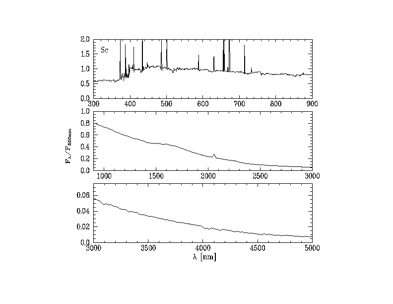
- Spiral (Sc) galaxy [plot, data] is a template spectrum (type Sc, class T=5) covering the wavelength range 22 - 10000 nm taken from the Pegase Atlas of Galaxies by Fioc & Rocca-Volmerange, 1997, A&A, 326, 950F. The spectrum has a sampling of 1nm at wavelengths shortwards of 878nm and 20nm longwards.
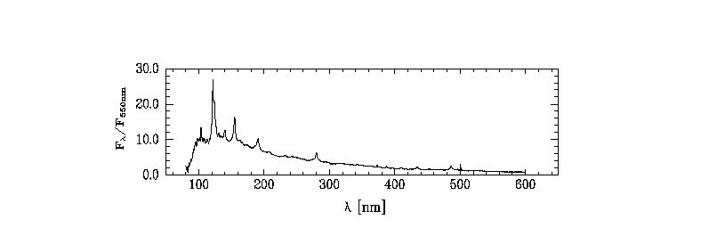
- QSO [plot, data] covers the (rest) wavelength range 80 - 855 nm with a spectral resolution ~1800 and a sampling of 0.1nm and is taken from Vanden Berk et al. 2001, AJ, 122, 549.
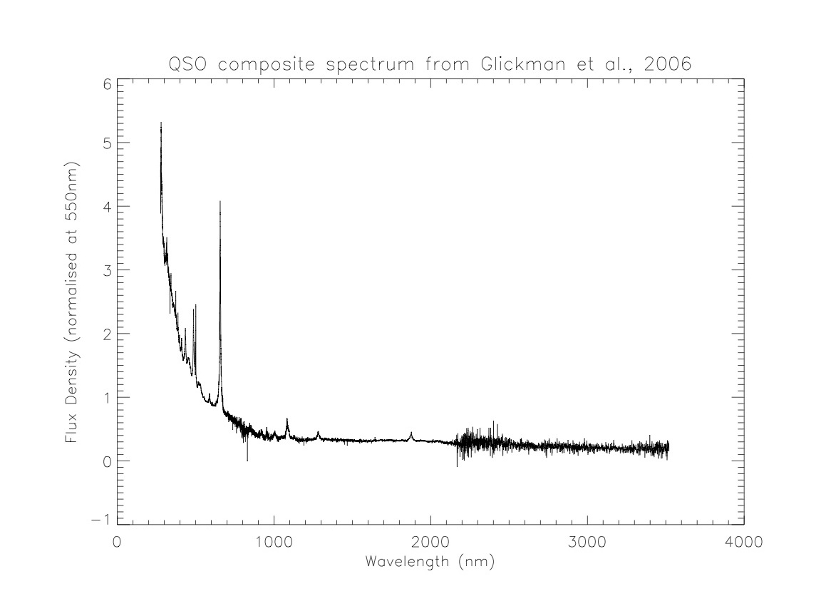
- QSO2 [plot, data] covers the (rest) wavelength range 276 - 3520 nm with a sampling of 0.1nm and is taken from Glikman et al. 2006, ApJ, 640, 579.
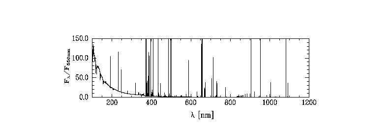
- HII region (Orion) [plot, data] covers the wavelength range 100 - 1100 nm with a sampling of 0.05nm and was taken from the HST STIS exposure time calculator.
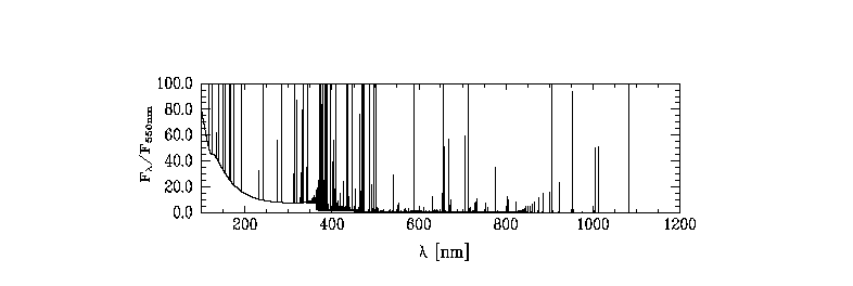
- Planetary nebula (NGC7009) [plot, data] covers the wavelength range 100 - 1100 nm with a sampling of 0.05nm and was taken from the HST STIS exposure time calculator.
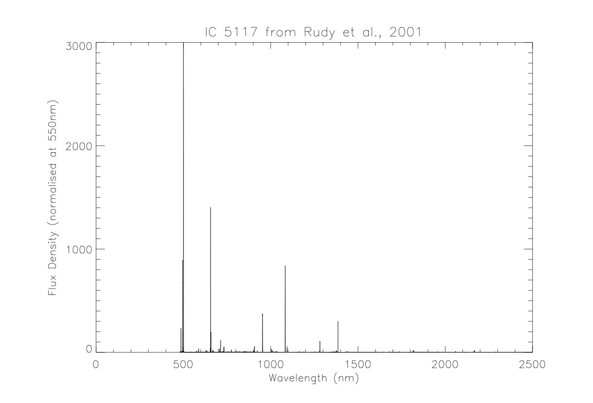
- Planetary nebula 2 (IC5117) [plot, data] covers the wavelength range 480 - 2500 nm with a sampling of 0.05nm and is taken from correspondence with Rick Rudy, based on Rudy et al. 2001, AJ, 121, 362.
(b) Mid-IR spectra:
A range of astronomical objects, including:
- Stellar spectra - types F-M, Wolf Rayets, carbon stars
- Other galactic objects - Galactic Centre, planetary nebula, pre-main-sequence star, young stellar object, reflection nebula, dusty HII region...
- Galaxy spectra - starburst nucleus, Seyfert II nucleus
(c) Stellar Libraries
The Pickles (1998; PASP, 110, 863) stellar library covers optical and near-IR wavelengths out to 2.5um across a broad range of spectral types (O5 to M9) and luminosity classes (I, III and V). We have extended these spectra out to 6um, arbitrarily adopting the slope of the K0III star for all spectral types. More accurate spectrophotometry will be inserted in the ITC library as it becomes available.
Model spectra for cool stars and brown dwarfs are provided from effective temperatures of 2800 K to 400 K. For temperatures down to 1200 K, the spectra are the version of BT-Settl models (Allard et al. 2012) that were used in the BHAC 2015 evolutionary models. Below 1200 K, the spectra are models from Morley et al. (2012) that have thin clouds (fsed=5). All models correspond to solar metallicity, and surface gravity is log(g) = 5.5 dex (cgs) down to 1800 K, 5.0 dex (cgs) down to 800 K, and 4.5 dex (cgs) down to 400 K.
(d) Single Emission Line and Continuum
This generates a Gaussian emission line on top of a flat (per wavelength interval) continuum. The specified line flux and continuum flux density override the brightness normalization defined as part of the spatial profile. If using a uniform surface brightness spatial profile the fluxes are per square arcsecond.
(e) User-Defined Spectrum
User-defined source spectra can be used instead of the existing template and model SEDs. Note the following restrictions on file format:
- Two columns separated by spaces:
- Wavelength in nm
- Flux density in arbitrary wavelength units, e.g. per nm or per um, but not per Hz
- Files may have any number of comment lines, each starting with the # character, and any number of blank lines.
- Wavelength interval need not be uniform.
- The wavelength range must extend to include both the full instrument coverage and the requested normalization filter (or wavelength). For example, a user-defined spectrum for T-ReCS must extend to below 2000nm if the source brightness is defined in the K-band.
- File size must be less than 1MB.
- File name must end in ".sed" when using the OT interface. The web interface also accepts files that end in ".txt" or ".dat"
Original version by Phil Puxley, Ted von Hippel, and Marianne Takamiya. Mid-IR spectra from Kevin Volk and Tom Geballe.
Adaptive Optics in the ITC
The ability of the AO system to correct the wavefront depends on the brightness and off-axis angle of the wavefront reference source (the AO "guide star"). The Strehl ratio of the AO-corrected core is approximated in the ITC by:
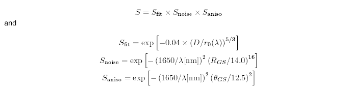
where Sfit is the Strehl due to the system fitting error (i.e. limited number of actuators), Snoise is the Strehl loss due to the limited number of photons from the guide star and Saniso is the Strehl loss due to anisoplantism. RGS is the R-band guide star magnitude and thetaGS is the off-axis angle in arcsec.
The total signal from a point source is the sum of the AO-corrected core and the uncorrected (seeing-limited) halo. For moderate or high Strehl ratios the core dominates, for poor correction (low Strehl) the halo dominates. As in the non-AO case, the ITC defaults to an "optimum" aperture which gives a reasonable approximation of the best S/N ratio; we have taken this to be 1.18 * FWHMAO, where FWHMAO is the width of the corrected core:
Last update August 29, 2003; Francois Rigaut and Phil Puxley
Observation Overheads
The ITC includes the following observation overheads: acquisitions (possibly more than one for long observations), detector readout, telescope offsetting, and re-centering of spectroscopic observations when required. These overheads are calculated for all instruments and modes except for GSAOI. These calculations make several assumptions about the observing strategy which may not apply to your program, so please review the results carefully.
Setup / Acquisition overheads are instrument and mode specific:
The ITC assumes one full acquisition for every 2 hours of science (where the 2 hours includes offsetting, readout, and DHS overheads, but excludes time for re-centering).
The ITC assumes one re-centering for these spectroscopic visits longer than 1 hour:
- Slit spectroscopy guided with PWFS
- GMOS IFU spectroscopy guided with PWFS where the S/N is <5 per exposure
- NIFS spectroscopy where the S/N is <5 per exposure
Offsetting overheads are based on the offset distance specified in the "Dither offset size" field of the ITC form. Slit spectroscopy assumes an ABBA offset pattern, while imaging and IFU spectroscopy assumes an ABAB offset pattern. Set the offset size to zero to if you are not planning on offsetting and these overheads will be excluded.
The ITC does NOT include overheads for partner calibrations like flats, arcs, or standard stars.
Telescope Properties
This page describes some telescope properties relevant to ITC calculations. See the Gemini telescope pages for more details.
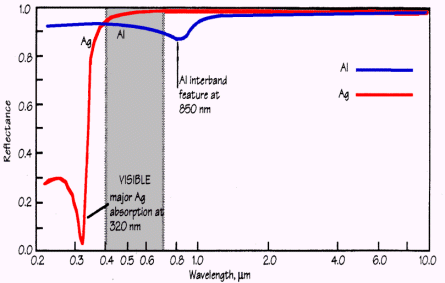
Mirror coating
The Gemini coating chamber is capable of depositing either alumini(u)m or silver. Currently the primary, secondary and tertiary (science fold) mirrors on both telescopes are silver coated. This graph shows the reflectivity of Al and Ag.
Instrument port
Gemini facility instruments may be mounted either on a side-looking or the up-looking ports of the instrument support structure (ISS). When mounted on a side port they are fed by reflection off the science fold mirror which incurs an additional small loss in transmission and an associated increase in emissivity. For signal-to-noise calculations it should be assumed that the instrument is side-looking. The default location for mid-IR instruments (e.g. T-ReCS, Michelle) is the up-looking port and is the side port for other instruments.
Wavefront sensor
Use of a peripheral wavefront sensor (PWFS) or an on-instrument wavefront sensor (OIWFS) is required to provide tip-tilt error signals for the image motion compensation by the secondary mirror. Not all instruments have an OIWFS; see the specific instrument pages for details. When present, the OIWFS allows selection of a WFS star closer to the science field and therefore usually provides better image motion compensation and smaller images (see the image quality section of the observing condition constraints page for more details).
Last update June 20, 2005; Phil Puxley
Observing Condition Constraints in the ITC
The observing condition constraints define the poorest conditions under which a queue-scheduled observation should be executed and indicate the conditions that can be expected by classically-scheduled observers. See the detailed translation between frequency of occurrence (the %-ile bin) and physical property, which is a function of observing wavelength and zenith distance of the source.
Within the ITC, the selected constraint determines which of several input files are loaded to define the sky transmission and emission, and the image size adopted for the nominal point source. Links to further details, or to the ASCII files themselves, are available here:
- Image quality (see the detailed translation for the meaning of the %-ile bins)
- The delivered image quality (not simply the seeing) is affected by many parameters including atmospheric properties (e.g. coherence length and time, scale length), wind speed and direction, guide star brightness and relative distance from target and observing wavelength. The tabulated values of image quality assume zenith pointing. As a first approximation, used in the ITC, the image size increases with air mass to the 3/5 power e.g. it is 50% larger at air mass = 2. The wavefront sensor employed for tip-tilt image motion compensation, either peripheral or on-instrument, is selected in the ITC as part of the telescope configuration.
- Sky transparency (cloud cover) (see the detailed translation for the meaning of the %-ile bins)
- Sky transparency (water vapour) (see the detailed translation for the meaning of the %-ile bins)
- optical (spectrum not yet available)
- near-IR (0.9-5.6µm coverage, resolution 1nm, sampled every 0.5nm). Selected spectra and data files are available for 20%-, 50%- and 80%-ile conditions at air masses of 1, 1.5 and 2.
- mid-IR (6-28µm coverage, resolution 1nm, sampled every 0.5nm). Selected spectra and data files are available for 20%-, 50%-, 80%-ile and "any" conditions at an air mass of 1.5.
- Sky background (see the detailed translation for the meaning of the %-ile bins)
- optical: spectrum not yet available
- near-IR: 0.9-5.6 µm coverage, resolution 2cm-1. An example spectrum and data file are available
- mid-IR: the water vapour column and airmass are taken into account by the ITC in calculating the mid-IR sky background, and it need not be explicitly defined here. The sky background should be set to "any" for mid-IR observations in the PIT and OT, except perhaps in cases where optically-dark skies are needed to guide on a faint guide star for a high-priority target.
- Air mass
- This is the typical air mass (i.e. 1 / cos[zenith distance]) expected during the observation.